 Table 7-1
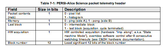
Table 7-1 The contents of the remainder of the data frames (the 32767-word data block) depend on the acquisition mode: - Pixel List: Each word in the data block from a pixel list exposure describes a photon event or a time hack. Photon events are indicated by bit 15 having a value of zero and time hacks are indicated by bit 15 having a value of one. For a photon event, the remaining 15 data bits encode the location of the detected event consisting of a 10-bit encoded spectral location (X) and a 5-bit encoded spatial location (Y). The time hack is used to provide temporal information about the photon events. The acquisition hardware will generate and insert time hacks in the frame on a periodic basis; the frequency of the time hacks is configurable (by command) for each acquisition in a range of 4 - 512 ms. For a time hack, the remaining 15 bits contain an incrementing counter that counts the number of 4 ms periods. This value allows for verification and correction of timing in case of lost frames or packets. - Histogram: Each word in the data block from a histogram exposure is a 16-bit "counter" giving the number of photon events detected at each specific X,Y location on the detector. The format of the detector is 1024x32 pixels, which are the spectral and spatial dimensions respectively, i.e., there are 1024 spectral elements along the X-axis and 32 spatial elements along the Y-axis, giving a total of 32768 values (however, the first word always contains the header word). The counters are stored row-wise, corresponding to the spectral dimension indexing most quickly. These counters saturate at a maximum value of 65535 to indicate a completely filled counting bin, meaning that the counters do not wrap around. In addition some special data words (header cross-identification and pulse height distribution) are overlying the lower left-hand corner of the actual array in a block of 4 (spatial) x 32 (spectral) words. This usage doesn't affect the science data contents because detector events do not occur in this region. In this over-written block, the first row contains the header cross-identification word, the second and third rows contain the 64 words of pulse height information, and the fourth row is filled with zeros. A "pulse height" is the amplitude of a photon event, and this pulse height distribution (PHD) shows the number of events in a 64-bin distribution with 6-bit resolution; the value in each PHD bin gives the number of events that occurred with the particular amplitude associated with that bin. These PHD counters also saturate at a value of 65535. So a single photon event is counted both in the spectral/spatial array and in the pulse height list. The PHD is used as a diagnostic for the health and behavior of the detector. For test purposes the instrument can fill the memory with known deterministic patterns so the interfaces to the spacecraft and ground can be verified. The instrument software allows for the generation of 5 different test patterns. 7.2.1.1 Histogram FITS file: The primary data unit in the FITS file is a 2-D raw histogram frame (also referred to as an "image") consisting of 1024x32 16-bit integer numbers. Note that the Alice instrument data are unsigned 16-bit integers (giving values of 0 to 65535). The first data extension in the FITS file contains the 64-element pulse height distribution (PHD) that was acquired together with the histogram. When the Level 1 pipeline saves the PHD to this extension, it then zeros out that part of the histogram array. The second data extension contains a 141 column by t row binary table, where t is the time of the exposure in seconds, of housekeeping values recorded during the observation (the housekeeping report rate is 1 Hz). FITS File Storage Location Description Primary Data Unit (PDU) Raw Histogram image (uncorrected counts) Extension #1 Pulse Height Distribution (PHD) Extension #2 Binary Housekeeping Table 7.2.1.2 Pixel list FITS file: Upon receiving a pixel list frame, the Level 1 processing creates a ground-calculated "reconstructed histogram" from the received pixel list data and places it in the primary data unit of the FITS file; this enables an easy quick-look inspection of the pixel list data (e.g., using most FITS viewers that by default typically display the data in the primary data unit). The pixel list data itself can be hard to interpret, so this reconstructed histogram image is desirable to enable the scientist to determine, e.g., data quality, whether the target was in the field of view, etc... The first data extension contains the raw pixel list data set, which includes the full stream of photon events and time hacks. The second extension contains the count rate derived from the pixels list data. Each count rate bin shows the number of events that occurred between successive time hacks. The resolution of this count rate data set is determined by the hack rate used for the pixel list acquisition. The length of this vector is variable depending on the source flux and the hack rate. The third data extension contains a 141 column by t row binary table, where t is the time of the exposure in seconds, of housekeeping values recorded during the observation. FITS File Storage Location Description Primary Data Unit (PDU) Reconstructed Histogram image (uncalibrated counts) Extension #1 7.2.1.3 raw pixel list Extension #2 7.2.1.4 Count rate vector from pixel list data (sampled at time hack rate) Extension #3 Binary Housekeeping Table 7.2.2 Data Sources (High/Low Speed, CCSDS, ITF) 7.2.2 Data Sources (High/Low Speed, CCSDS, ITF) PERSI-Alice data are transferred via CCSDS packets that are packetized 7.2.by the spacecraft from the Solid State Recorder. The spacecraft will packetize the PERSI-Alice High Speed Telemetry data into CCSDS packages before sending the data to the ground. Different APIDs are used to distinguish the histogram and pixel list data packets (see Table 7-2). For the PERSI-Alice science frames the spacecraft will either use the "RAW" packetized format or the loss-less compressed format to transfer the data. In either case the result will be data encoded in CCSDS telemetry packets. The package APIDs listed in Table 7-2 are used to distinguish the different Alice CCSDS packets. The packet time as listed in the CCSDS packet represents the time at which the packetization operation was performed. The second time field contains the frame collection time as sent from a spacecraft perspective, meaning this represents the time at which the spacecraft received the frame from the instrument. As the instrument immediately sends the frame at the completion of the acquisition this corresponds to the time at which the acquisition was completed.
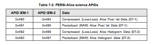 Table 7-2
Table 7-2: PERSI-Alice science APIDs Packetized "RAW" telemetry: The nominal data transfer method for the Alice pixel list science data is packetized "raw" data. Each CCSDS science packet can transfer a segment of up to 480 data bytes. In order to transfer a full PERSI-Alice frame of 32768 words (16-bits), 137 science packets are needed; the first 136 packets will all be full size segments of 480 bytes, the last packet will transfer the remaining 256 bytes. The grouping flags of the packets indicate the start and end segment within a complete frame transfer. Note the '#' marks in the following tables refer to the third digit of the APID, the valid digits for these numbers are indicated in Table 7-2.
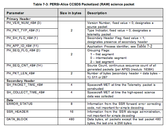 Table 7-3
Table 7-3: PERSI-Alice CCSDS Packetized (RAW) science packet Lossless Compressed telemetry: The nominal data transfer method for the Alice histogram science data is lossless compressed data. When applied to pixel list data, the 'FAST' algorithm results in negligible compression rates, and occasionally in a 1% expansion, therefore lossless compression will generally not be used with pixel list data. The spacecraft uses the so called 'FAST' algorithm to compress the image data. The 'FAST' algorithm uses one-dimensional correlation between successive data elements to remove redundancy. Data is encoded in blocks of 16 successive science values, the first value of such a block is send in full 16 bits, the remainder of the block is encoded using successive differences, using an adaptive coding mechanism.
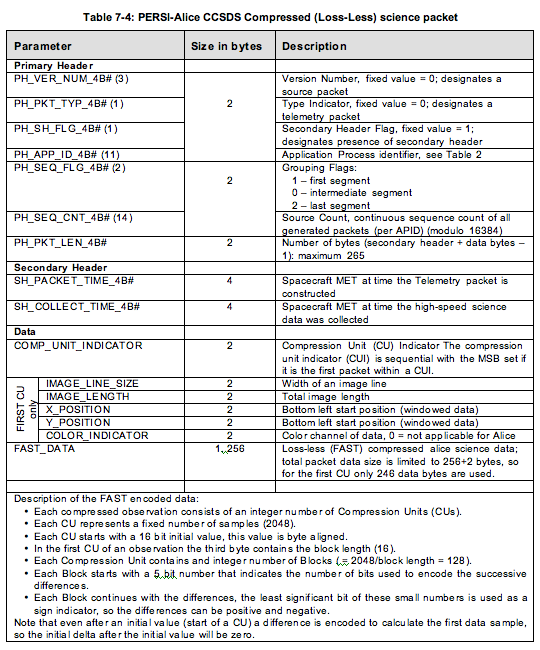 Table 7-4
Table 7-4: PERSI-Alice CCSDS Compressed (Loss-Less) science packet 7.2.3 Definition of an "Observation" An observation will be a single histogram image or one frame of a pixel list series. Each observation will be written to a separate FITS file. A pixel list resulting from a single exposure command may therefore produce many such frames, each of which will be saved as a separate FITS file. 7.2.4 S/C Housekeeping Needed in Level 1 Files (for Calibration) Spacecraft housekeeping that may be needed in the Alice pipeline include any temperature sensors on the spacecraft around the Alice instrument and the spacecraft-measured instrument bus voltage and power consumption on the different busses. Spacecraft measured temperatures related to Alice (ApId 0x00D and 0x08D): T_A.CDH_TEMP_ALICE_BRACK_BASE_00D T_A.CDH_TEMP_ALICE_1_00D T_A.CDH_TEMP_ALICE_2_00D PDU parameters related to Alice (ApId 0x009, 0x00a, 0x089 and 0x08a): ALICE_LVPS_A_VOLT_009 ALICE_LVPS_A_CURR_009 ALICE_LVPS_B_VOLT_009 ALICE_LVPS_B_CURR_009 ALICE_ACT_A_VOLT_00A ALICE_ACT_A_CURR_00A ALICE_ACT_B_VOLT_009 ALICE_ACT_B_CURR_009 Note that these temperatures currently are not used in the pipeline processing, but may be used in the future as the code and calibrations are revised. 7.3 "Calibrated" Data Specifics "Calibrated" data as used here refers to CODMAC level 3 data. 7.3.1 Algorithm for Pipeline Overview: The Alice calibration pipeline that is run at the SOC applies various calibrations to raw Alice data to convert the data from units of counts to flux units (photons/s/cm2). Four types of operations can be performed. They are, in order of application to the data: deadtime correction, dark correction, effective area correction, and flat field correction. These are described in more detail below. 7.3.1.1 Deadtime Correction The Alice detector electronics require a finite time to process a photoelectron pulse. As a result, if photoelectron pulses arrive too close together in time, the latter pulse(s) will not be recorded, resulting in an effective decrease in the sensitivity of the instrument that is a function of the count rate. The deadtime correction time constant is 18 microseconds. At input rates below 50 kHz, the detector electronics is non-paralyzable (fixed deadtime per event that is not re-triggerable). To calculate the detector output count rate, the following formula is used: C_out = C_in / (1 + C_in tau), where Cout is the output (i.e., detected) count rate and C_in is the input count rate. At a count rate of 1 kHz, the deadtime correction factor (tau) is approximately 1.02, while at 20 kHz, the deadtime correction factor is approximately 1.56. 7.3.1.2 Dark Correction The Alice detector electronics register photon events even when the aperture door is closed and the detector is not illuminated. The spatial distribution of dark counts is approximately uniform across the detector. However, there is some low-level 2-D structure to the dark counts. Alice observations made with the aperture door closed are summed together to create a "superdark". This superdark image is then scaled to the exposure time of an Alice science observation and subtracted from the data. During in-flight commissioning, these dark counts were measured at a rate of approximately 94 Hz across the entire detector. The primary source of dark counts is the spacecraft RTG. Dark exposures are made throughout the mission to monitor the background event rate and detector performance. 7.3.1.3 Effective Area The sensitivity of Alice to UV photons varies as a function of wavelength. It is convenient to think of the Alice sensitivity in terms of the effective area of the instrument. For a point source located at infinity, effective area is defined as the area of the surface that intercepts incident photons at the same rate as is detected by the Alice instrument. Dividing the observed count rate by the effective area yields the incident flux of photons. In general, effective area depends on the geometric size of the instrument aperture, reflectivities of the optical surfaces, sensitivity and quantum efficiency of the detector, etc. The Alice effective area curve (v003) is based on pre-flight estimates and calibration stars observed by both Alice and the IUE satellite. Above 1350 Angstroms, the effective area is derived from matching the stellar flux observed by Alice with that observed by IUE. Below 1350 Angstroms, the pre-flight effective area estimate has been scaled by a factor of 0.6 so that the long wavelength end of the pre-flight effective area estimate approximately matches the calibration derived from the stellar observations. 7.3.1.4 Flat Field When uniformly illuminated by a monochromatic source, the counts detected by the Alice instrument vary from pixel to pixel with a standard deviation of approximately 15%. This spatial variation in instrument sensitivity is the instrument flat field response. As of September 2007, no suitable observations have been made from which to derive an in-flight flat field calibration. Thus the flat field correction is currently disabled in the Alice pipeline code. Current plans are that during annual checkouts, a stellar scan along the slit could be used to generate a pseudo-flat field that could be used in the Alice pipeline. 7.3.2 Format of Calibrated Data 7.3.2.1 Histogram The primary data unit in the FITS file is a 2-D calibrated histogram frame consisting of 1024x32 array of 32-bit floating-point numbers. The units of the histogram image are photons/s/cm2. The first data extension in the FITS file is a 1024x32 array of 32-bit floating numbers containing the uncertainty in the histogram image. The second data extension is a 1024x32 element array containing the wavelength for each pixel in the histogram image. The third data extension is the 64-element PHD, identical to that in the raw data. The fourth data extension is an array containing the number of photon events per second, sampled at a rate of 1 Hz. The fifth data extension is the 141 column by t row housekeeping row as in the raw data. FITS File Storage Location Description Primary Data Unit (PDU) Calibrated Histogram image (photons/sec/cm2) Extension #1 Uncertainties in histogram data values Extension #2 Wavelength Image (Angstroms) Extension #3 Pulse Height Distribution (PHD) Extension #4 Count rate vector from HK (sampled at 1 Hz) Extension #5 Binary Housekeeping Table 7.3.2.2 Pixel List The primary data unit in the FITS file is a 2-D calibrated reconstructed histogram image consisting of a 1024x32 array of 32-bit floating-point numbers. The units of the histogram image are photons/s/cm2. The first data extension in the FITS file is a 1024x32 array of 32-bit floating numbers containing the uncertainty in the reconstructed histogram image. The second data extension is a 1024x32 element array containing the wavelength for each pixel in the reconstructed histogram image. The third data extension contains a binary table of 5 columns and rows for each photon event. The five columns are the X (spectral) position of each photon event, the Y (spatial) position of the photon event, the wavelength of the photon event, the cumulative number of elapsed time intervals (starting from 0 at the beginning of the file), and the ephemeris time (et), i.e. seconds past J2000, at the time of detection. The fourth data extension is the count rate derived from the pixels list data, showing the number of events that occurred between successive time hacks. The resolution of this count rate data set is determined by the hack rate used for the pixel list acquisition. The length of this vector is variable depending on the source flux and the hack rate. The fifth data extension contains the binary housekeeping table. FITS File Storage Location Description Primary Data Unit (PDU) Reconstructed Calibrated Histogram image (photons/sec/cm2) Extension #1 Uncertainties in reconstructed histogram data values Extension #2 Wavelength Image (Angstroms) Extension #3 Binary Pixel List Table (X, Y, wavelength, time hack #, MET) Extension #4 Count rate vector from pixel list data (sampled at time hack rate) Extension #5 Binary Housekeeping Table 7.3.3 7.3.3 Scientific Units For Histogram, units are counts (histogram), angstroms (wavelength array), and counts (PHD array). For Pixel List, units are counts (generated histogram), angstroms (wavelength array), counts, pixel location, and angstroms, and seconds (pixel list array), counts per second (count rate array). 7.3.4 Additional FITS and PDS Keywords Added Below is an example of the Mike pipeline keyword block added to the FITS header: COMMENT ============================================= COMMENT MIKE_BEG= 'Feb 15 16:12:57 2005' / START MIKE KEYWORD BLOCK MIKE_VER= '2.0 [2005 Feb 15]' /Version of Mike pipeline code K_MODE = 'ACQMODE ' / Keyword containing the mode name K_ETIME = 'EXPTIME ' / Keyword for the effective exposure time FILE_IN = 'test/ali_0000006498_0x4b3_eng_1.fit' / Input file for processing FILE_OUT= 'test/test_his.fit' / Output file after processing DIR_CAL = 'cal/ ' / Directory of calibration data DIR_DONE= ' ' / Directory to put raw data after processing BADFILE = ' ' / FITS file of bad pixel mask array BADFLAG = -1 / Bad pixel mask flag BADVALUE= -666 / Bad pixel value DEADFILE= 'deadtime/ra_dead_002.txt' / Deadtime correction file DEADFLAG= 1 / DEADTYPE= 'FUN ' / Correct using FUNction or lookup table (LUT)? DEADCORR= 'TOTAL ' / Correct by TOTAL or each PIXEL count rate? BIASFILE= ' ' / Bias image filename BIASFLAG= -1 / Bias correction flag DARKFILE= 'dark/ra_dark_001.fit' / Dark image filename DARKFLAG= -1 / Dark correction flag FLATFILE= 'flat/ra_flat_001.fit' / Flag field image filename FLATFLAG= -1 / Flat field correction flag FLATNORM= 'AVERAGE ' / How to normalize flat field WCALFLAG= 0 / Wavelength calibration flag WCALPRO = 'alice_wavecal' / IDL program to perform wavelength calibration WCALPARS= 'T_DELECC' / keywords for parameters to use for wave cal AEFFFLAG= 1 / AEFFPRO = 'alice_aeff' / IDL program to get effective area AEFFPARS= 'T_DELECC' / keywords for parameters to get effective area LOG_FILE= 'test/log.out' / Filename to save log file (default = append to LOG_MAIL= ' ' / address (if any) to e-mail log file MIKE_ERR= 1 / MIKE_END= 'Tue Feb 15 16:12:57 2005' / END MIKE KEYWORD BLOCK COMMENT ============================================= COMMENT 7.3.5 Hardware/OS Development Platform Dell Linux, Redhat 7.2; Apple G5 Power PC and PowerBook G4, OS X v10.4 7.3.6 Language(s) Used IDL 7.3.7 Third Party Libraries Required IDL Astro (http://idlastro.gsfc.nasa.gov/) 7.3.8 Predicted Execution time A few seconds per file. 7.3.9 Contact/Support Person(s) Andrew Steffl, Joel Parker, and Maarten Versteeg 8. LEISA INSTRUMENT DESCRIPTION 8.1 Overview LEISA is an infrared imaging spectrometer. The detector is a 256x256 pixel array. Spectral separation is done with a wedged optical etalon filter placed in close proximity to the detector array. The filter is made of two pieces, a high spectral resolution (lambda/delta(lambda)=580) segment and a low spectral resolution (lambda/delta(lambda)=280) segment, bonded together. The detector-filter assembly is located at the plane of focus of the Ralph telescope where a 2-D image is recorded simultaneously with the infrared spectrum of the scene. The layout for the filter assembly is shown in Figure 8-0: Layout for LVF Filter Assembly. The wavelength range of the sensor is 1.225-2.5 nm for the low resolution segment and 2.1-2.25 microns for the high resolution segment. The wavelength of transmission of the filter varies along one axis and is constant in the other. Lines of constant wavelength are aligned with the row direction of the detector array. The number of pixel-limited spectral channels is the number of rows of the detector, excluding a number of rows (4) obscured by opaque adhesive at the bond joint between the two filter segments.
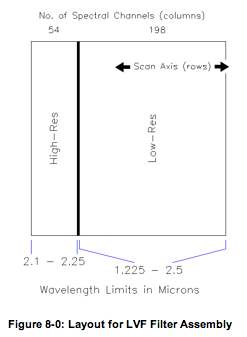 Figure 8-0: Layout for LVF Filter Assembly
The LEISA detector array is a Rockwell PICNIC device. It is read out
by the Ralph electronics in Correlated Double Sample (CDS) mode. The
signal is converted to a 12-bit value using the middle 12 bits of a 16
bit analog to digital (A/D) converter. There are two data transfer
modes, one in which both signal and reset level data are returned
(un-subtracted mode), and the other in which the reset level is
subtracted from the signal level and only the difference is returned
(subtracted mode).
The image cube is recorded as a series of N image frames, with N
determined by the length of the scan multiplied by the frame
rate. Detector frame rate is adjustable between 0.25 and 8 Hz in 1 ms
steps. Each frame covers the complete range of wavelengths. LEISA is
normally operated in a scanning mode, with the target moving through
the image plane, row by row. Slicing the image cube along one row
gives a scanned image of the target in one wavelength. Co-registering
each wavelength image (removing motion and optical distortion) yields
an IR spectrum of the target.
Data recorded on New Horizons is sent to the ground via the Deep Space
Network. From there the data is sent to the Mission Operations Center
(MOC) at the Applied Physics Laboratory (APL). The Science Operations
Center (SOC) retrieves new data from the MOC daily. The SOC software
pipelines convert the data from the MOC archives into FITS (Flexible
Image Transport) files with scientifically useful and calibrated
data. The SOC first sorts the packets into image cubes of raw (12-bit)
sensor counts with useful header keywords. These keywords include the
recording mode of the observation, timing information and basic
pointing information of the instrument boresight. The raw processing
also gathers housekeeping (H/K) telemetry from the Ralph instrument
into a table. Once the raw processing is complete, the SOC produced a
calibrated data set for each observation.
8.2 Raw Data Specifics
8.2.1 Data Format
Raw Dataset:
The SOC stores the LEISA data cubes in Band Interleaved by Line (BIL)
order, i.e. image frames are stored sequentially. To re-order LEISA
images as received from the spacecraft, the SOC does the following to
each frame of data:
1. de-interlace by quadrant
2. reverse the Y direction
3. rotate 180 degrees
The resulting frames from LEISA have the (0,0,0) element of the 3-D
array corresponds to the location of wavelength 2.5 microns on the LEISA
filter at the minimum X axis location in the image in the first
frame.
The SOC raw data product is a FITS format data file and PDS detached
label file. Ancillary data for an observation is placed in the primary
header of the FITS data file. The 256X256XN data cube is stored in
the primary data unit as an array of integers. The first FITS
extension is a binary table of Ralph housekeeping data.
Outline of the raw FITS file:
- Primary HDU - Raw 12 bit image counts
- Primary Header (FITS + pointing + observation keywords)
- 256 X 256 X N integer point array
- Extension 1 - Binary table of Ralph housekeeping
- Ext. Header (keywords + binary table definition)
- Ext. Binary Table (115 X S binary table of Ralph housekeeping data)
*[N is the number of data image frames in the observation, S is the
number of seconds in the observation]
**[In the case of un-subtracted readout mode, frames alternate between
read and reset signal levels]
Image Data
The primary data unit contains the raw spectral image data. Values
recorded by the instrument with 12 bit precision are stored as 16 bit
integers.
Housekeeping Data
Housekeeping data generated by the Ralph instrument is stored in
Extension 1 as a binary table. The first field in each row of the
table is mission elapsed tine (MET). Table entries are sorted by
increasing MET. The time interval between each table entry is fixed,
one second per entry, unless there is missing data. Pipeline
Processing
The limits of an observation are established by the SOC using
information in each telemetry packet of an observation sequence.
8.2.2 Data Sources (High/Low Speed, CCSDS, ITF)
Ralph housekeeping data is transmitted in the form of CCSDS packets.
One housekeeping packet is produced by the Ralph instrument each time
a spacecraft PPS (pulse per second) signal is received. State
information is gathered, time tagged, and written to the low speed bus
in CCSDS packet form. The CCSDS packets are transmitted during the
next DSN pass.
LEISA image data is transmitted in the form of CCSDS packets produced
by the spacecraft compression/packetization routines from the data
written to the high-speed bus. The LEISA detector has 4 output
channels, one for each array quadrant. The first 4 elements of the
data stream are the first pixels from each quadrant. The second 4
elements are the second pixels from each quadrant, and so on. One
'line' of data in this order is 4x 128 pixels long, and is not the
same as a line in the final image. During the observation, image data
is written to the spacecraft high speed bus. These data are not
automatically transmitted. A compression/packetization routine is
scheduled some time later that converts the Ralph sensor counts to a
packetized form.
The data can be packetized without compression, with lossless
compression, or with lossy JPEG compression. The packetization
routine can also process a sub-frame area of interest, or a more
complicated sliding subframe that tracks the image target as the
scanning observation proceeds. In un-subtracted readout mode, the
spacecraft interface supports only uncompressed downlink. Regardless
of windowing or compression, the SOC raw data processing reassembles
the data into a full 256X256XN data cube.
8.2.3 Definition of an "Observation"
Science Operation
The size of the LEISA detector is 256 x 256 pixels. One read out of
all 65,536 detector pixels is called an image or frame. The data
content of a LEISA "frame" is consistent with the S/C definition of
the term. The processing definition of "image" is consistent with the
optical definition except that the order of pixel elements is
different in the electronic data stream.
An observation is a sequence of frames. The number of frames per
observation is variable. Pixel values are recorded with 12 bit
precision. One image contains 65536 pixels x 1.5 bytes/pixel = 98304
bytes of data, however, data is stored as 16 bit values in the SOC
data files.
For normal science observations the Ralph electronics use the value of
the frame rate to minimize smearing by compensating for the spacecraft
motion and scan rate relative to the target. Reset levels are stored
temporarily by the electronics and subtracted from read levels
(subtracted mode). The difference in read and reset levels is
transferred to the spacecraft. Alternately, the instrument can be
forced to use a fixed frame rate value.
Un-subtracted Read-out:
There is a voltage offset for each LEISA quadrant to assure the sensor
signal will be in the correct range of the A/D. The offset values are
set from a table when Ralph is powered on. Un-subtracted mode can be
used to evaluate the offset values. In un-subtracted readout mode,
reset levels are not subtracted from read levels. Both read and reset
are transferred. The number of values in one data frame of the
un-subtracted mode (131,072) is 2x twice that of subtracted mode. Read
and reset values are interleaved by data line and the number and order
of the pixel elements in a line are the same as for subtracted mode
readout. The reset of a pixel occurs after the integrated signal is
read, so read levels correlate with reset levels recorded in the
preceding frame. The spacecraft interface supports only uncompressed
packetization of the full LEISA array for un-subtracted readout mode.
8.2.4 Housekeeping Needed in Level 1 Files (for Calibration)
Most of the H/K values are used for engineering troubleshooting and
not needed for data processing. Housekeeping data that are important
to further processing (see the following table) are stored in header
keywords.
Keyword Description
SIDE Instrument hardware side
DETECTOR Always LEISA for LEISA data
FILTER Always WEDGE for LEISA data
LEI_OFFx Value used to set voltage offsets for the four LEISA quadrants. x=1-4
LEI_RATE Time between LEISA readouts (ms)
8.2.5 Science Data and/or Housekeeping Requirements
Other important information is determined by the SOC while processing
the raw observation data. These values are also stored as keywords in
the FITS header.
Keyword Description
MET510 The MET of the Ralph housekeeping packet that marks the start
of an observation, used to determine the observation start time and
frame rate
TRUE510 Is the 0x510 real or assumed from a gap?
SCANTYPE Always LEISA for LEISA data
LEI_MODE RAW for un-subtracted readout mode
SUBTRACTED for subtracted readout mode
STARTMET Actual start time of first integration, in MET (s)
EXPTIME LEISA exposure time (s). Same as RALPHEXP.
There is zero dead time between frames so the
frame rate is exactly 1/EXPTIME
SPICE and SPICE Kernels:
The SOC maintains an archive of SPICE kernels that describe the
position and attitude of the spacecraft as any time in the mission.
The kernels are used to calculate many values describe the instrument
pointing during each observation, stored as header keywords with the
prefix SPC. The names of the SPICE kernels used to process the
observation are stored as header keywords with the prefix SPCK.
8.3 Calibrated Data Specifics
8.3.1 Algorithm for Pipeline
There are six processing steps applied to the raw LEISA data to produce the calibrated output:
1. Validate raw image file
2. Preprocess un-subtracted mode data
3. Process A/D rollover pixels
4. Convert raw counts to calibrated values
5. Compute pointing data
6. Construct FITS file
Validate raw image file
The input file is validated to assure the data is ready for further
8.processing. Checks are for valid mission, instrument, mode, and
8.image array size. The values of important keywords are validated
8.and collected in this step.
Preprocess un-subtracted mode data
If the data readout was in un-subtracted mode, the reset values are
subtracted from the read values in this step and the rest of the
processing is the same, regardless of readout mode.
Process A/D rollover pixels
There are two instances where the subtracted raw data value will be
off by exactly 4096 counts. The first is when the subtraction of the
reset count results in a negative number . This happens because of
array noise and read noise and results in small negative numbers being
returned as large positive number.s. The second instance is when the
subtraction of the reset count results in a number greater than 4095
(12 bits). This happens because the most significant bit of the A/D
is not read. A count higher than 4095 is normally considered outside
of dynamic range of LEISA, but can be corrected on a case by case
bases.
If a file identifying rollover pixels for the observation exists (see
next paragraph), the identified pixels are corrected for rollover. If
no file exists, any subtracted count greater than 3850 is considered
to have rolled over, and 4096 is subtracted from the raw count value.
This is a good first-cut since the observations will not be designed
to return signal counts this high.
During initial image analysis by the Ralph team, each observation is
analyzed in detail. A file identifying rollover pixels is generated
which identifies the pixels that are deemed to need rollover
correction. The case where the read count is higher than 4095 can be
detected by analyzing surrounding pixels and by watching the target
scan through the array. These are also included in the rollover file.
Once this file is installed on the SOC, processing of the calibrated
data for the observation will automatically use the rollover file
instead of the default processing.
Convert raw counts to calibrated values
There are 8 values that make up the conversion between raw signal
count and calibrated signal value.
1. Electronics induced readout signal
2. CCD flat field
3. Calibration offset
4. Calibration gain
5. Integration time
6. Filter width
7. Pixel solid angle
8. Gain correction
The electronics induced readout signal is a base signal that does not
depend on integration time. It has been derived from studies of the
dark frames of flight data and is subtracted from the raw signal
count.
The CCD flat field is derived from laboratory data and refined with in
flight observation data. The flat field changes slightly as the
mission progresses so a different flat field can be defined for an
individual observation or a range of observations. The actual flat
field used in the processing is included in the output FITS file.
The calibration offsets and calibration gains are derived from
laboratory data and refined with in flight observation data. These
values can change as the mission progresses. Different calibration
values can be defined for an individual observation or a range of
observations. The actual calibration values used in the processing
are included in the output FITS file.
The integration time is divided into the calculated calibrated counts.
The filter width of each pixel is divided into the calculated calibrated counts.
The pixel solid angle is divided into the calculated calibrated counts.
The gain correction is divided into the calculated calibrated counts.
All of these values are derived from laboratory data and refined with
in flight calibration observation data. They are updated, as needed
an applied to the observation data automatically when re-processed
Compute pointing data
The pointing for each pixel of each frame is computed using the timing
information from the observation, reconstructed ephemeris and attitude
files, and knowledge of the optical distortion of the instrument. One
array is generated giving the cartesian pointing vector of each pixel
in the LEISA array. This is a function only of the optical distortion
of the system. A second array is generated giving the rotation
quaternion of the instrument boresight into the J2000 reference frame
for the middle of each exposure. By rotating the pointing vector of a
pixel by the quaternion for the image frame, the J2000 pointing vector
of each pixel can be derived
Construct FITS files
A FITS file is constructed to store all the calibrated image data and related processing data.
8.3.2 Dataflow Block Diagram
Figure 8-0: Layout for LVF Filter Assembly
The LEISA detector array is a Rockwell PICNIC device. It is read out
by the Ralph electronics in Correlated Double Sample (CDS) mode. The
signal is converted to a 12-bit value using the middle 12 bits of a 16
bit analog to digital (A/D) converter. There are two data transfer
modes, one in which both signal and reset level data are returned
(un-subtracted mode), and the other in which the reset level is
subtracted from the signal level and only the difference is returned
(subtracted mode).
The image cube is recorded as a series of N image frames, with N
determined by the length of the scan multiplied by the frame
rate. Detector frame rate is adjustable between 0.25 and 8 Hz in 1 ms
steps. Each frame covers the complete range of wavelengths. LEISA is
normally operated in a scanning mode, with the target moving through
the image plane, row by row. Slicing the image cube along one row
gives a scanned image of the target in one wavelength. Co-registering
each wavelength image (removing motion and optical distortion) yields
an IR spectrum of the target.
Data recorded on New Horizons is sent to the ground via the Deep Space
Network. From there the data is sent to the Mission Operations Center
(MOC) at the Applied Physics Laboratory (APL). The Science Operations
Center (SOC) retrieves new data from the MOC daily. The SOC software
pipelines convert the data from the MOC archives into FITS (Flexible
Image Transport) files with scientifically useful and calibrated
data. The SOC first sorts the packets into image cubes of raw (12-bit)
sensor counts with useful header keywords. These keywords include the
recording mode of the observation, timing information and basic
pointing information of the instrument boresight. The raw processing
also gathers housekeeping (H/K) telemetry from the Ralph instrument
into a table. Once the raw processing is complete, the SOC produced a
calibrated data set for each observation.
8.2 Raw Data Specifics
8.2.1 Data Format
Raw Dataset:
The SOC stores the LEISA data cubes in Band Interleaved by Line (BIL)
order, i.e. image frames are stored sequentially. To re-order LEISA
images as received from the spacecraft, the SOC does the following to
each frame of data:
1. de-interlace by quadrant
2. reverse the Y direction
3. rotate 180 degrees
The resulting frames from LEISA have the (0,0,0) element of the 3-D
array corresponds to the location of wavelength 2.5 microns on the LEISA
filter at the minimum X axis location in the image in the first
frame.
The SOC raw data product is a FITS format data file and PDS detached
label file. Ancillary data for an observation is placed in the primary
header of the FITS data file. The 256X256XN data cube is stored in
the primary data unit as an array of integers. The first FITS
extension is a binary table of Ralph housekeeping data.
Outline of the raw FITS file:
- Primary HDU - Raw 12 bit image counts
- Primary Header (FITS + pointing + observation keywords)
- 256 X 256 X N integer point array
- Extension 1 - Binary table of Ralph housekeeping
- Ext. Header (keywords + binary table definition)
- Ext. Binary Table (115 X S binary table of Ralph housekeeping data)
*[N is the number of data image frames in the observation, S is the
number of seconds in the observation]
**[In the case of un-subtracted readout mode, frames alternate between
read and reset signal levels]
Image Data
The primary data unit contains the raw spectral image data. Values
recorded by the instrument with 12 bit precision are stored as 16 bit
integers.
Housekeeping Data
Housekeeping data generated by the Ralph instrument is stored in
Extension 1 as a binary table. The first field in each row of the
table is mission elapsed tine (MET). Table entries are sorted by
increasing MET. The time interval between each table entry is fixed,
one second per entry, unless there is missing data. Pipeline
Processing
The limits of an observation are established by the SOC using
information in each telemetry packet of an observation sequence.
8.2.2 Data Sources (High/Low Speed, CCSDS, ITF)
Ralph housekeeping data is transmitted in the form of CCSDS packets.
One housekeeping packet is produced by the Ralph instrument each time
a spacecraft PPS (pulse per second) signal is received. State
information is gathered, time tagged, and written to the low speed bus
in CCSDS packet form. The CCSDS packets are transmitted during the
next DSN pass.
LEISA image data is transmitted in the form of CCSDS packets produced
by the spacecraft compression/packetization routines from the data
written to the high-speed bus. The LEISA detector has 4 output
channels, one for each array quadrant. The first 4 elements of the
data stream are the first pixels from each quadrant. The second 4
elements are the second pixels from each quadrant, and so on. One
'line' of data in this order is 4x 128 pixels long, and is not the
same as a line in the final image. During the observation, image data
is written to the spacecraft high speed bus. These data are not
automatically transmitted. A compression/packetization routine is
scheduled some time later that converts the Ralph sensor counts to a
packetized form.
The data can be packetized without compression, with lossless
compression, or with lossy JPEG compression. The packetization
routine can also process a sub-frame area of interest, or a more
complicated sliding subframe that tracks the image target as the
scanning observation proceeds. In un-subtracted readout mode, the
spacecraft interface supports only uncompressed downlink. Regardless
of windowing or compression, the SOC raw data processing reassembles
the data into a full 256X256XN data cube.
8.2.3 Definition of an "Observation"
Science Operation
The size of the LEISA detector is 256 x 256 pixels. One read out of
all 65,536 detector pixels is called an image or frame. The data
content of a LEISA "frame" is consistent with the S/C definition of
the term. The processing definition of "image" is consistent with the
optical definition except that the order of pixel elements is
different in the electronic data stream.
An observation is a sequence of frames. The number of frames per
observation is variable. Pixel values are recorded with 12 bit
precision. One image contains 65536 pixels x 1.5 bytes/pixel = 98304
bytes of data, however, data is stored as 16 bit values in the SOC
data files.
For normal science observations the Ralph electronics use the value of
the frame rate to minimize smearing by compensating for the spacecraft
motion and scan rate relative to the target. Reset levels are stored
temporarily by the electronics and subtracted from read levels
(subtracted mode). The difference in read and reset levels is
transferred to the spacecraft. Alternately, the instrument can be
forced to use a fixed frame rate value.
Un-subtracted Read-out:
There is a voltage offset for each LEISA quadrant to assure the sensor
signal will be in the correct range of the A/D. The offset values are
set from a table when Ralph is powered on. Un-subtracted mode can be
used to evaluate the offset values. In un-subtracted readout mode,
reset levels are not subtracted from read levels. Both read and reset
are transferred. The number of values in one data frame of the
un-subtracted mode (131,072) is 2x twice that of subtracted mode. Read
and reset values are interleaved by data line and the number and order
of the pixel elements in a line are the same as for subtracted mode
readout. The reset of a pixel occurs after the integrated signal is
read, so read levels correlate with reset levels recorded in the
preceding frame. The spacecraft interface supports only uncompressed
packetization of the full LEISA array for un-subtracted readout mode.
8.2.4 Housekeeping Needed in Level 1 Files (for Calibration)
Most of the H/K values are used for engineering troubleshooting and
not needed for data processing. Housekeeping data that are important
to further processing (see the following table) are stored in header
keywords.
Keyword Description
SIDE Instrument hardware side
DETECTOR Always LEISA for LEISA data
FILTER Always WEDGE for LEISA data
LEI_OFFx Value used to set voltage offsets for the four LEISA quadrants. x=1-4
LEI_RATE Time between LEISA readouts (ms)
8.2.5 Science Data and/or Housekeeping Requirements
Other important information is determined by the SOC while processing
the raw observation data. These values are also stored as keywords in
the FITS header.
Keyword Description
MET510 The MET of the Ralph housekeeping packet that marks the start
of an observation, used to determine the observation start time and
frame rate
TRUE510 Is the 0x510 real or assumed from a gap?
SCANTYPE Always LEISA for LEISA data
LEI_MODE RAW for un-subtracted readout mode
SUBTRACTED for subtracted readout mode
STARTMET Actual start time of first integration, in MET (s)
EXPTIME LEISA exposure time (s). Same as RALPHEXP.
There is zero dead time between frames so the
frame rate is exactly 1/EXPTIME
SPICE and SPICE Kernels:
The SOC maintains an archive of SPICE kernels that describe the
position and attitude of the spacecraft as any time in the mission.
The kernels are used to calculate many values describe the instrument
pointing during each observation, stored as header keywords with the
prefix SPC. The names of the SPICE kernels used to process the
observation are stored as header keywords with the prefix SPCK.
8.3 Calibrated Data Specifics
8.3.1 Algorithm for Pipeline
There are six processing steps applied to the raw LEISA data to produce the calibrated output:
1. Validate raw image file
2. Preprocess un-subtracted mode data
3. Process A/D rollover pixels
4. Convert raw counts to calibrated values
5. Compute pointing data
6. Construct FITS file
Validate raw image file
The input file is validated to assure the data is ready for further
8.processing. Checks are for valid mission, instrument, mode, and
8.image array size. The values of important keywords are validated
8.and collected in this step.
Preprocess un-subtracted mode data
If the data readout was in un-subtracted mode, the reset values are
subtracted from the read values in this step and the rest of the
processing is the same, regardless of readout mode.
Process A/D rollover pixels
There are two instances where the subtracted raw data value will be
off by exactly 4096 counts. The first is when the subtraction of the
reset count results in a negative number . This happens because of
array noise and read noise and results in small negative numbers being
returned as large positive number.s. The second instance is when the
subtraction of the reset count results in a number greater than 4095
(12 bits). This happens because the most significant bit of the A/D
is not read. A count higher than 4095 is normally considered outside
of dynamic range of LEISA, but can be corrected on a case by case
bases.
If a file identifying rollover pixels for the observation exists (see
next paragraph), the identified pixels are corrected for rollover. If
no file exists, any subtracted count greater than 3850 is considered
to have rolled over, and 4096 is subtracted from the raw count value.
This is a good first-cut since the observations will not be designed
to return signal counts this high.
During initial image analysis by the Ralph team, each observation is
analyzed in detail. A file identifying rollover pixels is generated
which identifies the pixels that are deemed to need rollover
correction. The case where the read count is higher than 4095 can be
detected by analyzing surrounding pixels and by watching the target
scan through the array. These are also included in the rollover file.
Once this file is installed on the SOC, processing of the calibrated
data for the observation will automatically use the rollover file
instead of the default processing.
Convert raw counts to calibrated values
There are 8 values that make up the conversion between raw signal
count and calibrated signal value.
1. Electronics induced readout signal
2. CCD flat field
3. Calibration offset
4. Calibration gain
5. Integration time
6. Filter width
7. Pixel solid angle
8. Gain correction
The electronics induced readout signal is a base signal that does not
depend on integration time. It has been derived from studies of the
dark frames of flight data and is subtracted from the raw signal
count.
The CCD flat field is derived from laboratory data and refined with in
flight observation data. The flat field changes slightly as the
mission progresses so a different flat field can be defined for an
individual observation or a range of observations. The actual flat
field used in the processing is included in the output FITS file.
The calibration offsets and calibration gains are derived from
laboratory data and refined with in flight observation data. These
values can change as the mission progresses. Different calibration
values can be defined for an individual observation or a range of
observations. The actual calibration values used in the processing
are included in the output FITS file.
The integration time is divided into the calculated calibrated counts.
The filter width of each pixel is divided into the calculated calibrated counts.
The pixel solid angle is divided into the calculated calibrated counts.
The gain correction is divided into the calculated calibrated counts.
All of these values are derived from laboratory data and refined with
in flight calibration observation data. They are updated, as needed
an applied to the observation data automatically when re-processed
Compute pointing data
The pointing for each pixel of each frame is computed using the timing
information from the observation, reconstructed ephemeris and attitude
files, and knowledge of the optical distortion of the instrument. One
array is generated giving the cartesian pointing vector of each pixel
in the LEISA array. This is a function only of the optical distortion
of the system. A second array is generated giving the rotation
quaternion of the instrument boresight into the J2000 reference frame
for the middle of each exposure. By rotating the pointing vector of a
pixel by the quaternion for the image frame, the J2000 pointing vector
of each pixel can be derived
Construct FITS files
A FITS file is constructed to store all the calibrated image data and related processing data.
8.3.2 Dataflow Block Diagram
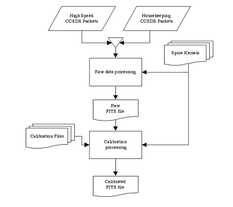 Figure 8-1: Dataflow Block Diagram
8.3.3 Data Format
Calibrated Dataset
The calibrated LEISA data are stored in Band Interleaved by Line (BIL)
order, exactly as the raw data is stored. The resulting frames from
LEISA have the (0,0,0) element of the 3-D array corresponds to the
location of wavelength 2.5 microns on the LEISA filter at the minimum X
axis location in the image in the first frame.
The calibrated data product is a FITS format data file and PDS
detached label file. Ancillary data for an observation is placed in
the primary header of the FITS data file. The 256X256XN data cube is
stored in the primary data unit as an array of floating point numbers.
The FITS extensions are outlined below.
Outline of the calibrated FITS file:
- Primary HDU - Calibrated image data
- Primary Header (FITS + pointing + observation keywords)
- 256 X 256 X N floating point array
- Extension 1 - Center wavelength and filter width for each pixel
- 256 X 256 X 2 floating point array
- Extension 2 - Cartesian pointing vector for each pixel
- 256 X 256 X 3 floating point array
- Extension 3 - Flat field correction for each pixel
- 256 X 256 X 1 floating point array
- Extension 4 - Radiometric gain and offset for each pixel
- 256 X 256 X 2 floating point array
- Extension 5 - Error estimates for each pixel
- 256 X 256 X 1 floating point array
- Extension 6 - Data quality flags for each pixel
- 256 X 256 X 1 Integer array
- Extension 7 - Ephemeris time and quaternion for each frame
- 5 X N floating point array
- Extension 8 - Binary table of Ralph housekeeping
- Ext. Header (keywords + binary table definition)
- Ext. Binary Table (115 X S binary table of Ralph housekeeping data)
*[N is the number of data image frames in the observation, S is the
number of seconds in the observation]
For a description of the contents of the FITS extension, see the above
section describing the SOC calibration processing.
Calibrated Image Data
The Image Data Unit of the Level 2 file contains data expressed in
physical units useful for scientific interpretation. The instrument
pipeline converts the data values of raw instrument counts to
radiance units, W/cm2/sr.
Data quality flags
The data quality flag is set if there is a known problem with the
given pixel.
Quality Flag Value Description
0 Good pixel
1 Defect in one of the calibration files
2 Flat field out of bounds
4 Known CCD defect
32 Bad pixel not in any of above categories
8.3.4 Extra FITS Extensions (planes) and Their Definitions
See above
8.3.5 Scientific Units
Radiometric units: W/cm2/sr
8.3.6 Additional FITS and PDS Keywords Added
See above
8.3.7 Hardware/OS Development Platform
The software for processing the raw and calibrated data files has been developed on the SOC computers, running GNU/Linux/i686 Version 2.6.17-1.2142_FC4.
8.3.8 Language(s) Used
The software for processing the raw data files is written in Python.
The software for processing the calibrated data files is written in C, with a Perl script wrapper.
8.3.9 Third Party Libraries Required
Python SPYCE interface library
Python MySQLdb interface library
Independent JPEG Group's JPEG software
CSPICE processing library
CFITSIO processing library
8.3.10 Calibration Files Needed (with Quantities)
The instrument software package will include additional datasets needed for calibrating the data. All The calibration software requires additional datasets needed for calibrating the data, as describe in the above sections. The instrument pipeline maintains version control on calibration datasets, as with calibration procedures. Some calibration files are associated with specific observations, some are associated with a range of observations.
The estimated number of calibration files needed for the mission is 300, totaling 3 GBs.
8.3.11 Memory Required
500MB
8.3.12 Temporary File System Space Needed
500MB
8.3.13 Predicted Size of Output File(s)
Up to 500MB
8.3.14 Predicted Execution time
Processing time for raw data files is approximately 3 seconds per image frame.
Processing time for calibrated data files is approximately .1 seconds per frame
8.3.15 Contact/Support Person(s)
Allen Lunsford
Dennis Reuter 301-286-2042
Donald Jennings 301-286-7701
Laddawan Miko 301-286-2166
8.3.16 Maintenance Schedule (Code/Data Updates, Documentation)
The LPS is installed by extracting files from an archive. The
sub-directory structure for the software package is created during
extraction. Symbolic links to external directories may be substituted
for default directory references. The shell for execution of the LPS
is tcsh/csh. Changes will be made to shell initialization files; new
elements are appended. Instructions for configuring the shell
environment are given. A guide to installation and setup is included
with the LPS package.
An initial period of testing and refinements is expected. Pieces of
the software are tested separately during development. LPS modules are
re-tested upon installation to the SOC. Sample datasets are provided
to verify the function of software. Integrated testing of the
instrument pipeline under the control of the SOC MDM is performed in
accordance with the SOC. The instrument software engineer is available
exclusively to the SOC to support the integration of pipeline
software.
Changes to calibration datasets are made as needed. A facility is
provided by the SOC so that software changes are reversible. A LEISA
team member will be available to assist SOC operators in responding to
unexpected errors in the instrument pipeline. Persons supporting the
LEISA Instrument Pipeline software are listed above.
The LEISA instrument pipeline is developed at GSFC. The first fully
functional version (v0) of the software is tested on the GSFC computer
system. In advance of completion of LPS v0, a skeleton software
package will be made available to the SOC. The skeleton software is a
callable code set which installs and functions as the instrument
pipeline but does not perform calibration and book keeping on
instrument data. Completion of software Version 0 encompasses the
creation of instrument calibration files. Documentation including
instructions for installation and setup will be delivered to the SOC
with Version 1 of the LPS. Updates of software after Version 1 are
performed on an as needed basis.
Figure 8-1: Dataflow Block Diagram
8.3.3 Data Format
Calibrated Dataset
The calibrated LEISA data are stored in Band Interleaved by Line (BIL)
order, exactly as the raw data is stored. The resulting frames from
LEISA have the (0,0,0) element of the 3-D array corresponds to the
location of wavelength 2.5 microns on the LEISA filter at the minimum X
axis location in the image in the first frame.
The calibrated data product is a FITS format data file and PDS
detached label file. Ancillary data for an observation is placed in
the primary header of the FITS data file. The 256X256XN data cube is
stored in the primary data unit as an array of floating point numbers.
The FITS extensions are outlined below.
Outline of the calibrated FITS file:
- Primary HDU - Calibrated image data
- Primary Header (FITS + pointing + observation keywords)
- 256 X 256 X N floating point array
- Extension 1 - Center wavelength and filter width for each pixel
- 256 X 256 X 2 floating point array
- Extension 2 - Cartesian pointing vector for each pixel
- 256 X 256 X 3 floating point array
- Extension 3 - Flat field correction for each pixel
- 256 X 256 X 1 floating point array
- Extension 4 - Radiometric gain and offset for each pixel
- 256 X 256 X 2 floating point array
- Extension 5 - Error estimates for each pixel
- 256 X 256 X 1 floating point array
- Extension 6 - Data quality flags for each pixel
- 256 X 256 X 1 Integer array
- Extension 7 - Ephemeris time and quaternion for each frame
- 5 X N floating point array
- Extension 8 - Binary table of Ralph housekeeping
- Ext. Header (keywords + binary table definition)
- Ext. Binary Table (115 X S binary table of Ralph housekeeping data)
*[N is the number of data image frames in the observation, S is the
number of seconds in the observation]
For a description of the contents of the FITS extension, see the above
section describing the SOC calibration processing.
Calibrated Image Data
The Image Data Unit of the Level 2 file contains data expressed in
physical units useful for scientific interpretation. The instrument
pipeline converts the data values of raw instrument counts to
radiance units, W/cm2/sr.
Data quality flags
The data quality flag is set if there is a known problem with the
given pixel.
Quality Flag Value Description
0 Good pixel
1 Defect in one of the calibration files
2 Flat field out of bounds
4 Known CCD defect
32 Bad pixel not in any of above categories
8.3.4 Extra FITS Extensions (planes) and Their Definitions
See above
8.3.5 Scientific Units
Radiometric units: W/cm2/sr
8.3.6 Additional FITS and PDS Keywords Added
See above
8.3.7 Hardware/OS Development Platform
The software for processing the raw and calibrated data files has been developed on the SOC computers, running GNU/Linux/i686 Version 2.6.17-1.2142_FC4.
8.3.8 Language(s) Used
The software for processing the raw data files is written in Python.
The software for processing the calibrated data files is written in C, with a Perl script wrapper.
8.3.9 Third Party Libraries Required
Python SPYCE interface library
Python MySQLdb interface library
Independent JPEG Group's JPEG software
CSPICE processing library
CFITSIO processing library
8.3.10 Calibration Files Needed (with Quantities)
The instrument software package will include additional datasets needed for calibrating the data. All The calibration software requires additional datasets needed for calibrating the data, as describe in the above sections. The instrument pipeline maintains version control on calibration datasets, as with calibration procedures. Some calibration files are associated with specific observations, some are associated with a range of observations.
The estimated number of calibration files needed for the mission is 300, totaling 3 GBs.
8.3.11 Memory Required
500MB
8.3.12 Temporary File System Space Needed
500MB
8.3.13 Predicted Size of Output File(s)
Up to 500MB
8.3.14 Predicted Execution time
Processing time for raw data files is approximately 3 seconds per image frame.
Processing time for calibrated data files is approximately .1 seconds per frame
8.3.15 Contact/Support Person(s)
Allen Lunsford
Dennis Reuter 301-286-2042
Donald Jennings 301-286-7701
Laddawan Miko 301-286-2166
8.3.16 Maintenance Schedule (Code/Data Updates, Documentation)
The LPS is installed by extracting files from an archive. The
sub-directory structure for the software package is created during
extraction. Symbolic links to external directories may be substituted
for default directory references. The shell for execution of the LPS
is tcsh/csh. Changes will be made to shell initialization files; new
elements are appended. Instructions for configuring the shell
environment are given. A guide to installation and setup is included
with the LPS package.
An initial period of testing and refinements is expected. Pieces of
the software are tested separately during development. LPS modules are
re-tested upon installation to the SOC. Sample datasets are provided
to verify the function of software. Integrated testing of the
instrument pipeline under the control of the SOC MDM is performed in
accordance with the SOC. The instrument software engineer is available
exclusively to the SOC to support the integration of pipeline
software.
Changes to calibration datasets are made as needed. A facility is
provided by the SOC so that software changes are reversible. A LEISA
team member will be available to assist SOC operators in responding to
unexpected errors in the instrument pipeline. Persons supporting the
LEISA Instrument Pipeline software are listed above.
The LEISA instrument pipeline is developed at GSFC. The first fully
functional version (v0) of the software is tested on the GSFC computer
system. In advance of completion of LPS v0, a skeleton software
package will be made available to the SOC. The skeleton software is a
callable code set which installs and functions as the instrument
pipeline but does not perform calibration and book keeping on
instrument data. Completion of software Version 0 encompasses the
creation of instrument calibration files. Documentation including
instructions for installation and setup will be delivered to the SOC
with Version 1 of the LPS. Updates of software after Version 1 are
performed on an as needed basis.
 Table 8-1
Table 8-1 9. LORRI INSTRUMENT DESCRIPTION 9.1 Overview The LOng Range Reconnaissance Imager (LORRI) is a narrow angle (FOV=0.29degrees), high resolution (IFOV=5 microrad), Ritchey-Chretien telescope with a 20.8 cm diameter primary mirror, a focal length of 263 cm, and a three lens field-flattening assembly. A 1024 x 1024 pixel (optically active region), back-thinned, backside-illuminated CCD detector (model CCD 47-20 from E2V) is located at the telescope focal plane and is operated in standard frame-transfer mode. LORRI does not have any color filters; it provides panchromatic imaging over a wide bandpass extending approximately from 350 nm to 850 nm. The LORRI telescope has a monolithic silicon carbide structure, built by SSG Precision Optronics, Inc., is designed to maintain focus over the entire operating temperature range (-125 C to +40 C) without a focus adjustment mechanism. A detailed description of the design and fabrication of LORRI can be found in the paper by Conard, et al., "Design and fabrication of the New Horizons Long-Range Reconnaissance Imager" in SPIE proceedings 5906-49, 2005. A detailed discussion of the performance of LORRI, as measured during calibration testing before launch, can be found in the paper by Morgan et al., "Calibration of the New Horizons Long-Range Reconnaissance Image" in SPIE proceedings 5606-49, 2005. LORRI is a supplemental instrument on New Horizons and is not needed to meet the baseline scientific objectives of the mission. Nevertheless, LORRI adds significant capabilities to New Horizons, including the highest available spatial resolution (50 m/pixel at the Pluto closest approach distance of 10,000 km) and redundancy for the primary optical imager, MVIC on Ralph. The exposure time for LORRI is adjustable in 1 msec increments from 0 ms to 29,967 msec. However, exposure times will normally be limited to < 150 msec to prevent image smear associated with spacecraft motion during observations. Initially, the shortest useful exposure time was expected to be ~40 msec owing to frame transfer smear associated with the transfer of charge from the active CCD region to the storage region, during which time the active region remains exposed to the image scene because LORRI has no shutter, but an improved frame transfer smear removal algorithm was developed that now permits exposure times as little as 1 msec. The LORRI exposure time can be commanded to a specific value, or LORRI can be operated in "auto-exposure" mode, in which the LORRI flight software sets the exposure time automatically based on the signal level in a previous image. In auto-exposure mode, the algorithm used to set the exposure time depends on several adjustable parameters that are stored in an onboard table. The optimal values for these table parameters vary with the type of scene being observed, which means that new table loads may be required prior to some observations. Although the LORRI auto-exposure mode worked well during ground testing, no decision has yet been made on whether it will be used in-flight during encounter observations. LORRI can also be operated in "rebin" mode, in which case the signal in a 4 x 4 pixel region is summed on-chip to produce an active region that is effectively 256 x 256 pixels covering the entire 0.29 degrees FOV. The main purpose of this mode is to provide high sensitivity acquisition of a Kuiper Belt object (KBO), which requires an exposure time of ~10 sec. Although LORRI rebin mode may never be used for science observations, the LORRI pipeline is still required to calibrate rebinned images.
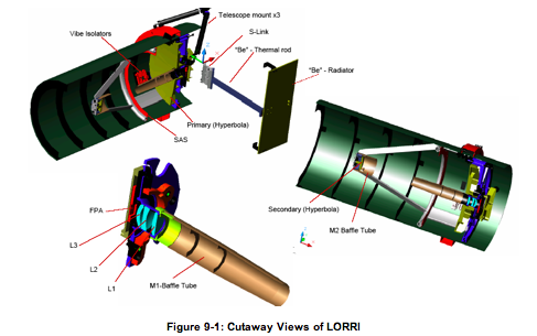 Figure 9-1: Cutaway Views of LORRI
9.2 Raw image Specifics
9.2.1 Data Format
The raw image data is organized in a FITS file. The primary header
9.and data unit (HDU) is used to store the reconstructed image from
9.telemetry. Additional data are stored in the extensions of the
9.file. The two tables below contain a description of the layout for
9.the extensions for raw data.
As described previously, LORRI operates in two binning modes: 1x1 and
4x4. For the 1x1 binning mode, the raw image dimensions are 1028x1024
where columns 0 through 1023 are the optically active region of the
CCD and the remaining columns (1024-1027) are from optically inactive
region (dark columns) of the CCD and represent a temperature-specific
measurement of the bias value. For the 4x4 binning mode, the raw
image dimensions ar 257 x 256 where columns 0 through 255 are
optically active and column 256 for the dark column.
Figure 9-1: Cutaway Views of LORRI
9.2 Raw image Specifics
9.2.1 Data Format
The raw image data is organized in a FITS file. The primary header
9.and data unit (HDU) is used to store the reconstructed image from
9.telemetry. Additional data are stored in the extensions of the
9.file. The two tables below contain a description of the layout for
9.the extensions for raw data.
As described previously, LORRI operates in two binning modes: 1x1 and
4x4. For the 1x1 binning mode, the raw image dimensions are 1028x1024
where columns 0 through 1023 are the optically active region of the
CCD and the remaining columns (1024-1027) are from optically inactive
region (dark columns) of the CCD and represent a temperature-specific
measurement of the bias value. For the 4x4 binning mode, the raw
image dimensions ar 257 x 256 where columns 0 through 255 are
optically active and column 256 for the dark column.
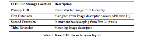 Table 9-5
Table 9-5: Raw FITS file extension layout 9.2.2 Data Sources (High/Low Speed, CCSDS, ITF) The LORRI high-rate data is delivered to the Instrument Interface card over a low-voltage differential signal (LVDS) interface and is then transferred to the SSR through the spacecraft high-speed PCI bus by the C&DH software. The image data is stored directly on the SSR and packets are generated by command to the C&DH software as is described in the table below. The APID from which the image originated is part of the filename, so this mapping may provide some assistance in decoding the filenames retrieved from the SOC.
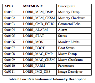 Table 9-6
Table 9-6: Low Rate Instrument Telemetry Description
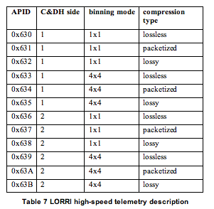 Table 9-7
Table 9-7: LORRI high-speed telemetry description 9.2.3 Definition of an "Observation" Each LORRI image is an "observation." 9.2.4 Housekeeping Needed in Raw Image Files (for Calibration) No special requirements other than pointing 9.2.5 Raw Science Data and/or Housekeeping Requirements No special requirements 9.3 Calibrated Image Specifics 9.3.1 Algorithms for Pipeline Calibration Process The calibration of LORRI images potentially involves all of the following steps: 1) Bias subtraction 2) Signal linearization 3) Charge transfer inefficiency (CTI) correction 4) Dark subtraction 5) Smear removal 6) Flat-fielding 7) Absolute calibration Ground testing has demonstrated that the linearization, CTI, and dark subtraction steps will not be needed, so they are not described below. Nevertheless, the LORRI pipeline architecture will be maintained to allow these additional steps to be incorporated quickly, if in-flight data suggest they are needed. The LORRI pipeline software consists of a series of IDL routines that implement the above processing steps. In general, the IDL routines have the following naming convention: lorri_function.pro, where "function" refers to the specific task performed by that routine. (The "pro" extension will be omitted below when discussing specific routines.) Each routine typically has several command line arguments and keywords that specify the input and output files and, possibly, parameters for tailoring the routine for particular circumstances. The routines that perform the bias subtraction, the smear removal, and the flat-fielding are described below. No special routines are provided to perform the absolute calibration. Instead, the absolute calibration is performed using keywords provided in the FITS header, as described further in Section 9.3.1.4. 9.3.1.1 Bias Subtraction If an image has an associated "dark" image (i.e., an image taken with the same exposure time but without any illumination), then the debiased image is simply the difference of those two images. This was usually the case during on-ground testing when images taken of a scene were immediately followed by images taken with the scene blocked (i.e., an obstruction was placed in the optical path to block the illumination). However, in-flight images may often be taken without accompanying darks either because of limitations on downlink bandwidth, or because a decision is made to take more target images at the expense of concurrent darks. In either case, the same pipeline routine will be used to debias the image (lorri_debias), but the algorithm employed is different in each case and different reference files are required. If in-flight data indicate that bias images are stable over time, many bias images will be combined (after filtering out clearly discrepant pixels) to produce a "super-bias" image. Then the median value of the inactive region of the image (i.e., the median of a 1024 row by 4 column region) is subtracted from the super-bias image to produce a "delta-bias" image. The IDL procedure that produces the delta-bias image is called lorri_delta_bias, but this routine is not part of the standard LORRI calibration pipeline; rather, it is an ancillary routine used to produce a calibration reference file. The delta-bias image will exhibit the pixel-to-pixel variation in the bias and will oscillate about zero. The bias subtraction for any new image is then a two-step process: 1) The median signal level in the inactive region of the image is subtracted from each pixel's value to remove the overall bias level, and 2) The delta-bias image is subtracted from the image created in the previous step to remove the pixel-to-pixel variation and produce the final, debiased image. Ground calibration testing showed that the overall bias level in step (1) above depends on the signal level in the last few columns of the active region of the CCD. The effect is produced by amplifier undershoot, which means that the bias level recorded by the pixels in the inactive region is smaller than the actual bias level. The magnitude of the effect depends on the signal level in the active region and on the column number in the inactive region and can be as large as ~12 DN. Thus, prior to computing the median signal in the inactive region (step 1 above), the intensities of all the pixels must be corrected for amplifier undershoot. This correction step is incorporated into the lorri_debias procedure. If the in-flight bias images vary significantly in time, separate bias images (i.e., 0 ms exposures) must be taken for each science image obtained. In this case, the bias subtraction proceeds exactly as performed during ground calibration testing, with the bias removal achieved by simple subtraction of the bias image from the science image. There are several drawbacks to this approach: (1) more images must be taken, which affects the data volume that must be stored on the on-board solid-state recorder, (2) more data must be downlinked, which may not be possible because of limited downlink bandwidth and/or the cost associated with the extra Deep Space Network (DSN) support required, (3) the signal-to-noise ratio (SNR) may be degraded because the bias subtraction no longer involves a high SNR reference file, and (4) fewer science images can be obtained because they have been displaced in the observing timeline by extra bias images. 9.3.1.2 Smear Removal LORRI does not have a shutter, so the target being observed illuminates the active region of the CCD whenever LORRI is pointed at the scene. In particular, the CCD continues to record the scene as the charge is transferred from the active portion to the storage area, and this results in a smearing of the observed scene. Fortunately, this smear can be removed to high accuracy using the correction algorithm described below. When bright objects are observed, the readout smear makes the raw image difficult to use for analysis purposes. In the image of Jupiter below, the raw image is on the left and the calibrated image with readout smear (aka frame transfer smear) removed is on the right.
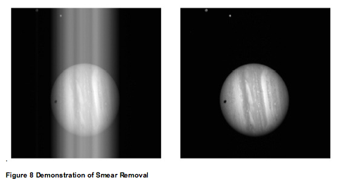 Figure 9-8: Demonstration of Smear Removal
The need for the readout smear removal arises from the operation of
the frame transfer CCD used in LORRI, where first the image zone is
flushed, then an exposure is taken, and finally the image is
transferred into the storage zone. Hence a pixel of the raw image is
exposed to the scene radiance from the corresponding geometrical
element of the scene, but it is also exposed to the radiances of all
the scene elements in the same image column during the image
transfers. Thus the raw image is the superposition of the scene
radiance and the signal acquired during frame transfers, which is
called readout smear.
The readout smear is removed as follows.
Equation 9-1
Figure 9-8: Demonstration of Smear Removal
The need for the readout smear removal arises from the operation of
the frame transfer CCD used in LORRI, where first the image zone is
flushed, then an exposure is taken, and finally the image is
transferred into the storage zone. Hence a pixel of the raw image is
exposed to the scene radiance from the corresponding geometrical
element of the scene, but it is also exposed to the radiances of all
the scene elements in the same image column during the image
transfers. Thus the raw image is the superposition of the scene
radiance and the signal acquired during frame transfers, which is
called readout smear.
The readout smear is removed as follows.
Equation 9-1
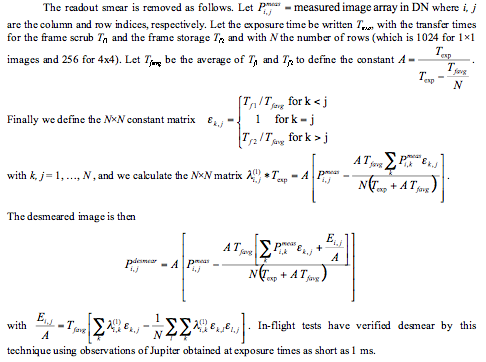 Equation 9-1
The value for T_favg is dependent on the desired exposure time and has been determined empirically using in-flight data. The following table provides the appropriate values at different exposure times.
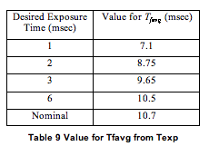 Table 9-9
Table 9-9 Value for T_favg from T_exp It should be noted that when the raw data is saturated, the resulting readout smear correction will be inaccurate. The algorithm relies on an accurate accumulation of charge in all rows of each column and if the raw data is clipped for lack of dynamic range to capture that integrated signal, the effect of readout smear cannot be completely and properly removed. This correction algorithm has been implemented in the IDL routine lorri_desmear. 9.3.1.3 Flat-Fielding Flat-fielding refers to the process of removing the pixel-to-pixel sensitivity variations in the image. An exposure obtained by illuminating the LORRI aperture uniformly with light is called a "flat-field" image. During ground calibration testing, flat-fields were obtained by using an "integrating sphere to provide uniform illumination. The light source was a xenon arc lamp with a spectrum similar to that of the sun. The absolute intensity of the input illumination was measured using a calibrated photodiode. For the panchromatic case, which is the one most relevant for flat-fielding LORRI images, the light from the xenon lamp was unfiltered. Flat-field images were also obtained by passing the light through bandpass filters centered at five different wavelengths spanning the range over which LORRI is sensitive, prior to injection into the reference sphere, in order to estimate the sensitivity of the flat-fields to the spectral distribution of the source. The spatial patterns in the flat-field images change fairly dramatically with wavelength. However, the variation in panchromatic flat-fields caused by differences in the spectral distribution of the illumination source should be much less significant. Indeed, panchromatic flat-field images produced using a tungsten lamp were virtually indistinguishable from those produced by the xenon lamp. Flat-fields were obtained at four different telescope temperatures (at standard laboratory room temperature, and at the lowest, nominal, and highest temperatures predicted for in-flight conditions), but no significant temperature variations in the flat-field images were detected. The flat-field reference file used in the LORRI pipeline was produced by averaging 100 flat-field images taken at room temperature using the xenon arc lamp as the light source, debiasing and desmearing the average image as described earlier, and normalizing the intensities in the active region to a median value of 1. If "S" (units are DN) is an image of a target that has already been desmeared and debiased, and if "FF" is the reference flat-field image, then the flat-fielded (i.e., photometrically-corrected) target image ("C"; units are DN) is given by: C = S/FF The flat-fielding correction is implemented in the LORRI pipeline by the routine lorri_flatten. If in-flight measurements indicate that the LORRI flat-field characteristics are different than those measured during ground calibration tests, new reference flat-field images must be obtained. Although LORRI has two internal reference lamps (sometimes referred to as "cal lamps"), the illumination pattern is highly non-uniform and, thus, not very suitable as a secondary flat-field standard. Various test measurements will be performed during the early portion of the mission to determine if scattered sunlight can serve as a suitable secondary flat-field standard. If there is a Jupiter encounter, smeared images of Jupiter might also prove to be useful as a secondary flat-field standard. In any case, there will be an attempt to monitor the flat-field characteristics of LORRI over time, and the reference flat-field image used by the LORRI pipeline will be updated as necessary to maintain an accuracy better than 1% in the correction of the pixel-to-pixel sensitivity variation, except possibly near the center of the field where image ghosts may compromise the quality of the reference flat-field (see further discussion below). During ground calibration tests, intensity artifacts caused by optical ghosts were observed near the center (roughly covering a 200 x 200 pixel region) of the flat-field images. Ray tracing of the optical system indicates that the intensity of the ghost image should be less than ~1% of the intensity produced by the direct illumination, but measurements indicated that ghost intensities have an amplitude of ~5-7% of the direct intensity for panchromatic illumination. The ghost intensity is scene-dependent with most (~80%) of the ghost signal arising from regions outside the nominal field-of-view of LORRI. There is a suspicion that at least some of the ghost signal is an artifact of the test conditions, and the reference flat-fields currently used by the pipeline do not include the ghost signal produced by the out-of-field light. Any flat-field data taken in-flight will be carefully scrutinized to search for any effects attributable to optical ghosts. Depending on those results, further modifications to the reference flat-fields may be required. There is also the possibility that different flat-field reference images may be required depending on the scene being imaged (i.e., a ghost subtraction step may be required prior to application of the flat-field correction under some circumstances). 9.3.1.4 Absolute Calibration (Conversion from corrected DN to physical units) The calibration software pipeline does not perform the conversion from DN to physical units because that conversion requires knowledge of the spectral distribution(i.e. color) of the target. Instead, various LORRI FITS header keywords ("photometry" keywords) are provided that allow users to convert from DN to physical units depending on the spectral type and spatial distribution (diffuse vs. point source) of the target. Photometry keywords are provided for targets having spectral distributions similar to Pluto, Charon, Pholus, Jupiter, and the Sun. The units adopted for the radiance (aka "intensity") of diffuse targets are ergs/cm2/s/sr/Angstrom. The units adopted for the irradiance (aka "flux") of point (i.e., unresolved) targets are ergs/cm2/s/Angstrom. Tables providing the values for the photometry keywords at the time of launch are given below. The latest (i.e., current) values of the photometry keywords are provided in the header of the calibrated image FITS file for the image being analyzed. The absolute calibration is achieved by specifying a keyword (RPLUTO) in the header of the calibrated image file that allows the user to convert a count rate ("C/TEXP" in DN/s/pixel, where "C" is the flat-fielded signal in a pixel and "TEXP" is the exposure time) for a resolved source into a radiance value ("I" in ergs/cm2/s/sr/Angstrom) at LORRI's pivot wavelength (specified by the FITS keyword PIVOT; see below), assuming that the spectrum of the target is identical to the globally-averaged spectrum of Pluto. The relevant formula is: I = C/TEXP/RPLUTO Similarly, the keyword RSOLAR allows the conversion of the count rate for a resolved source into a radiance value at the pivot wavelength assuming that the target has a solar-like spectral distribution: I = C/TEXP/ RSOLAR Finally, the keyword RPHOLUS allows the conversion of the count rate for a resolved source into a radiance value at the pivot wavelength assuming that the target has a spectral distribution identical to that of the centaur object 5145 Pholus, which may be a good analog for the reddest regions on Pluto: I = C/TEXP/RPHOLUS The current best estimates for these sensitivity keywords, based on ground calibration tests, are provided in the table below. In-flight calibration observations of photometric standard stars will be used to verify these values and to monitor them over time. Keyword Value [(DN/s/pixel)/(ergs/cm^2/s/sr/Angstrom)] RSOLAR 2.664 x 10^5 RPLUTO 2.575 x 10^5 RCHARON 2.630 x 10^5 RJUPITER 2.347 x 10^5 RPHOLUS 3.243 x 10^3 If users need conversions for other spectral distributions, they must derive those themselves using the LORRI spectral response function provided in the paper describing LORRI's in-flight calibration results. The pivot wavelength (PIVOT) is given by Equation 9-2, where "P" is
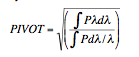 Equation 9-2
the LORRI system quantum efficiency (i.e., fraction of photons detected) at wavelength " lambda". The current best estimate for the LORRI pivot wavelength is 6076 Angstroms. For unresolved sources (e.g., stars), the absolutely calibrated flux (also called "irradiance") at the pivot wavelength can be determined using keywords that are defined analogously to the photometry keywords discussed above for resolved sources. In the case of a source having a spectral distribution identical to that of a globally-averaged Pluto spectrum, the observed count rate integrated over the LORRI PSF ("CINT/TEXP" in DN/s, where CINT is the total number of flat-field corrected counts integrated over the image and "TEXP" is the exposure time) can be related to the flux ("F" in ergs/cm2/s/Angstrom) by: F = CINT/TEXP/PPLUTO Similarly, the flux at the pivot wavelength for a target having the same spectral distribution as the sun is given by: F = CINT/TEXP/PSOLAR And the flux at the pivot wavelength for a target having the same spectral distribution as 5145 Pholus is given by: F = CINT/TEXP/PPHOLUS The current best estimates for these sensitivity keywords, based on ground calibration tests, are provided in the table below. In-flight calibration observations of photometric standard stars will be used to verify these values and to monitor them over time. Keyword Value [(DN/s)/(ergs/cm2/s/Angstrom)] PSOLAR 1.066 x 10^16 PPLUTO 1.030 x 10^16 PCHARON 1.052 x 10^16 PJUPITER 9.386 x 10^16 PPHOLUS 1.297 x 10^16 Synthetic photometry techniques can be used to convert the fluxes derived in the manner described above to fluxes at other wavelengths, and then into standard UBVRI magnitudes in the Landolt (1992) photometric system, which is essentially identical to the Johnson UBV system combined with the Kron-Cousins RI system. The results described in the LORRI calibration paper can be used to derive fluxes for targets whose spectral distributions do not match the three cases discussed above. We provide below some examples showing how to convert from engineering units to physical units, for both diffuse and point targets. Consider a diffuse target whose spectrum is similar to that of Pluto. You should then use the RPLUTO photometry keyword in the header of the calibrated image file to convert a count rate ("C/TEXP" in DN/s/pixel, where "C" is the flat-fielded signal in a pixel and "TEXP" is the exposure time) into a radiance value ("I" in ergs/cm2/s/sr/Angstrom) at LORRI's "pivot" wavelength (specified by the FITS keyword PIVOT for the formal definition of the pivot wavelength): I = C/TEXP/RPLUTO Similarly, the photometry keywords RSOLAR, RCHARON, RJUPITER, and RPHOLUS should be used to convert count rates into radiance values at the pivot wavelength assuming that the target has, respectively, solar-like, Charon-like, Jupiter-like, or Pholus-like spectral distributions. For LORRI, the pivot wavelength is 6076.2 Angstroms, and we don't expect this to change, at least not significantly. Since the solar flux (F_solar) at a heliocentric distance of 1 AU at the pivot wavelength is 176 erg/cm2/s/Angstrom, the value for the radiance can be converted to I/F (where pi*F = F_solar) using: I/F = pi * I * r^2 / F_solar where "r" is the target's heliocentric distance in AU. For unresolved targets (e.g., stars), the absolutely calibrated flux (also called the "irradiance") at the pivot wavelength can be determined using keywords that are defined analogously to the photometry keywords discussed above for resolved targets. In the case of a target having a spectral distribution identical to that of a globally-averaged Pluto spectrum, the observed count rate integrated over the LORRI PSF ("CINT/TEXP" in DN/s, where CINT is the total number of flat-field corrected counts integrated over the image and "TEXP" is the exposure time) can be related to the flux ("F" in ergs/cm2/s/Angstroms; not to be confused with "F" in I/F) by: F = CINT/TEXP/PPLUTO When observing point targets, it is more common to convert the absolute flux to a magnitude in a standard photometric system. The following equation can be used to transform a measured value of the irradiance (aka "flux") of an unresolved target to a magnitude in the standard V band: V = -2.5 log S + PHOTZPT + CC + BC where "V" is the visual magnitude in the Johnson photometric system, PHOTZPT is the "stellar photometry keyword", which is the "zero point" of the LORRI instrumental magnitude system, "S" is the integrated net signal rate from the target in DN/s, "CC" is the color correction (i.e., correction for the spectral distribution of the target), and "BC" is the aperture correction (in case the flux is not integrated over the entire stellar image; a careful analysis of the flux versus aperture size for a bright star in the field can then be used to determine the value of BC for the aperture selected for the photometry). In-flight photometry of stars in the open galactic cluster M7 yield the following: PHOTZPT = 18.94
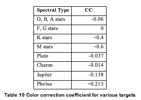 Table 9-10
Table 9-10: Color correction coefficient for various targets The following reference flux information is provided for convenience and was gathered from several sources. The UBV are in the Johnson system, RI are in the Landolt-Kron-Cousins system, and JHK_sK are in the UKIRT system. The fluxes for Vega are from the model STScI absolutely-calibrated spectrum. At near-IR wavelengths, the model underestimates the actual Vega flux by about 5-6% owing to the excess flux from the Vega dust disk. Note also that Vega has U=B=V=0.03 (i.e., not 0).
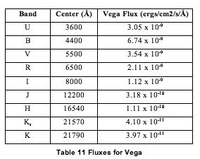 Table 9-11
Table 9-11 Fluxes for Vega 9.3.1.5 Pointing Information Pointing information for the LORRI boresight (center of the LORRI field-of-view, which is pixel [511,511]) is included in the FITS header in both the raw and the calibrated image files. An example of this information follows: SPCBLRA = 233.4199004768138 / [degrees] Boresight RA, EME J2000 SPCBLDEC= -17.96897170490819 / [degrees] Boresight DEC, EME J2000 SPCEMEN = 283.935414259362 / [degrees] EME J2k North Clk Angle, CW from UP 9.3.1.6 Conversion of instrument housekeeping items to engineering units The LORRI-specific housekeeping items reported in the raw FITS file are in units of counts or DN. To make these values more useful for data analysis, they have been converted to engineering units (volts, amps, degrees Celsius) and reported at the tail end of the header of the primary HDU of the calibrated FITS file. Because the contents of the raw header are duplicated in the calibrated file, a different set of tag names are used for the values that have been converted to engineering units. The new tags are reported after the comment that reads "LORRI Level 2 Calibrated telemetry items". 9.3.2 Instrument Characterization There are several characteristics of the instrument that are related to the radiometric calibration of LORRI that will be useful when analyzing the calibrated image data. They are the quantum efficiency and spectral responsivity, each as a function of wavelength. There are tables for each of these in the calibration directory for the PDS archive, but a graph for each is reproduced in the figures below.
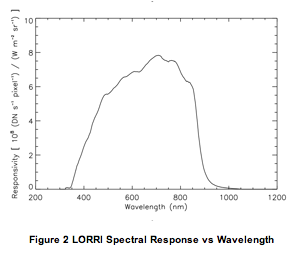 Figure 9-2: LORRI Spectral Response vs Wavelength
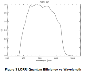 Figure 9-3: LORRI Quantum Efficiency vs Wavelength
After the data have been calibrated, additional processing steps are
likely to be required. Obvious examples of this are ghost removal and
stray light processing. At present, there have been no algorithms
developed for public release because they are highly scene dependent.
Individual images must be analyzed to understand the structure of the
effects to determine an appropriate method for its removal. In the
example below, a cutout from a calibrated image is presented to
illustrate the effect of stray light from Jupiter's disk, which is
just out of the field of view. The circular structure is an example
of the ghost pattern. The image on the right demonstrates the
processed version of that image. The gradient from the stray light has
been removed, as well as the majority of the effects of the ghost.
Figure 9-3: LORRI Quantum Efficiency vs Wavelength
After the data have been calibrated, additional processing steps are
likely to be required. Obvious examples of this are ghost removal and
stray light processing. At present, there have been no algorithms
developed for public release because they are highly scene dependent.
Individual images must be analyzed to understand the structure of the
effects to determine an appropriate method for its removal. In the
example below, a cutout from a calibrated image is presented to
illustrate the effect of stray light from Jupiter's disk, which is
just out of the field of view. The circular structure is an example
of the ghost pattern. The image on the right demonstrates the
processed version of that image. The gradient from the stray light has
been removed, as well as the majority of the effects of the ghost.
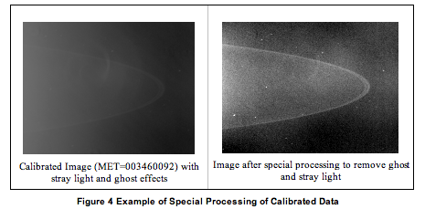 Figure 9-4 Example of Special Processing of Calibrated Data
9.3.4 Dataflow Block Diagram
Figure 9-4 Example of Special Processing of Calibrated Data
9.3.4 Dataflow Block Diagram
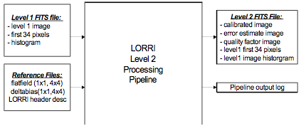 Figure 9-5
9.3.5 Data Format
The calibrated image data is organized in a FITS file. The primary
header and data unit (HDU) is used to store the calibrated image that
results from the calibration pipeline. The first extension is the
error estimate image, followed by the second extension containing the
data quality image. The table below contains a description of the
layout for the extensions for calibrated data.
For 1x1 binning mode, the calibrated image dimensions are 1024x1024,
and for 4x4 mode, the dimensions are 256x256 pixels. In both
situations, these pixels correspond to the optically active pixels
from the raw image mentioned previously.
Figure 9-5
9.3.5 Data Format
The calibrated image data is organized in a FITS file. The primary
header and data unit (HDU) is used to store the calibrated image that
results from the calibration pipeline. The first extension is the
error estimate image, followed by the second extension containing the
data quality image. The table below contains a description of the
layout for the extensions for calibrated data.
For 1x1 binning mode, the calibrated image dimensions are 1024x1024,
and for 4x4 mode, the dimensions are 256x256 pixels. In both
situations, these pixels correspond to the optically active pixels
from the raw image mentioned previously.
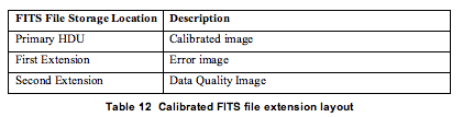 Table 9-12
Table 9-12 Calibrated FITS file extension layout LORRI calibrated FITS files have 3 extensions. The debiased, desmeared LORRI image is written into the primary HDU as a 2-dimensional, 32-bit real image. The unit for each data value is photometrically-corrected DN. The estimated errors in these corrected DN values are stored as a 2-dimensional, 16-bit real image in the first extension. A data quality image is stored in the second extension as a 2-dimensional, 16-bit integer image. The error in the photometrically-corrected signal is estimated from Equation 9-3, where "sigma" is the 1-sigma error in the corrected signal
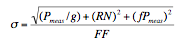 Equation 9-3
for a particular pixel (DN), "Pmeas" is the observed signal in that pixel (DN, after bias subtraction but before smear removal), "g" is the electronics gain (22 e/DN), "RN" is the electronics noise (1.3 DN), "f" is the estimated error in the reference flat-field image (0.005), and "FF" is the value of the reference flat-field image at the relevant pixel. The above formula neglects any noise contributed by the bias and smear removal steps, but those errors are generally expected to be small compared to the other sources of error. The data quality image is used to flag pixels that have known artifacts and may need special consideration when performing scientific analysis. The pixel value in the quality flag image represents the sum of all quality flags present for that pixel. This pixel value can also be described as the result of the bitwise 'OR' of each quality flag value. The list of data quality values and their descriptions are listed in Table 9-13.
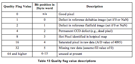 Table 9-13
Table 9-13 Quality flag value descriptions 9.3.7 Scientific Units Following the convention adopted by the New Horizons Principal Investigator, the unit used for calibrated data product are "photometrically-corrected DN". The procedure given above must be completed to obtain absolutely calibrated data products. The units adopted for the radiance ( aka "intensity") of diffuse targets are ergs/cm2/s/sr/Angstroms. The units adopted for irradiance (aka "flux") of point (i.e. unresolved) targets are ergs/cm2/s/Angstroms. Wavelengths are quoted in angstrom units. 9.3.8 Additional FITS and PDS Keywords Added Listed below are the keywords and sample values for those keywords that have been added to the FITS header and are stored with the primary HDU of the output calibrated image FITS file. COMMENT ********************************************************* COMMENT *** LORRI Level 2 software name and version info *** COMMENT ********************************************************* L2_SWNAM= 'lorri_level2_pipeline' /Level 2 calibration software L2_SWVER= 'untagged' /software version tag COMMENT ********************************************************* COMMENT *** LORRI Level 2 software logic flow control flags *** COMMENT ********************************************************* IMGSUBTR= 'OMIT ' / image subtraction step BIASCORR= 'PERFORM ' / bias subtraction step SLINCORR= 'OMIT ' / signal linearization step CTICORR = 'OMIT ' / charge transfer inefficiency step DARKCORR= 'OMIT ' / dark subtraction step SMEARCOR= 'PERFORM ' / smear removal step FLATCORR= 'PERFORM ' / flat-fielding step GEOMCORR= 'OMIT ' / geometric correction step ABSCCORR= 'PERFORM ' / absolute calibration step COMPERR = 'PERFORM ' / compute error estimate COMPQUAL= 'PERFORM ' / compute quality flags COMMENT ********************************************************* COMMENT *** LORRI Level 2 Reference Filename *** COMMENT ********************************************************* REFDEBIA= 'sap_006_combined_100img_1x1.fit' / debias image filename REFFLAT = 'cflat_grnd_SFA_20050309_v2.fit' / flat field image filename REFDEAD = 'dead_ground_1x1_synthetic.fit' / dead pixel image filename REFHOT = 'hot_ground_1x1_synthetic.fit' / hot pixel image filename REFSUBIM= ' ' / subtraction image filename COMMENT ********************************************************* COMMENT *** LORRI Level 2 Absolute Calibration Parameters *** COMMENT ********************************************************* PIVOT = 6076.20019531 / LORRI pivot wavelength. units=angstroms RSOLAR = 266400.000000 / Conv to radiance for solar source RPLUTO = 257500.000000 / Conv to radiance for pluto source RPHOLUS = 324300.000000 / Conv to radiance for 5145 pholus source RCHARON = 263000.000000 / Conv to radiance for charon source RJUPITER= 234700.000000 / Conv to radiance for jupiter source PPLUTO = 1.03000005170E+16 / Conv to irradiance for pluto source PSOLAR = 1.06600003807E+16 / Conv to irradiance for solar source PPHOLUS = 1.29700002225E+16 / Conv to irradiance for 5145 pholus source PCHARON = 1.05199994793E+16 / Conv to irradiance for charon source PJUPITER= 9.38600033786E+15 / Conv to irradiance for jupiter source PHOTZPT = 18.9400000000 / Zero point for visual magnitude, V COMMENT ********************************************************* COMMENT *** LORRI Level 2 Calibrated telemetry items *** COMMENT ********************************************************* EPU_P5VO= 5.04305504857 / EPU +5 voltage. units=Volts EPU_P5CU= 0.143143000000 / EPU +5 current. units=Amps FPU_P15V= 15.0005851594 / FPU +15 voltage. units=Volts FPU_P15C= 0.0493827000000 / FPU +15 current. units=Amps FPU_P6_V= 6.05666080780 / FPU +6 voltage. units=Volts FPU_P6_C= 0.152152000000 / FPU +6 current. units=Amps FPU_HTRC= 0.00000000000 / FPU heater current. units=Amps EPU_25PV= 2.50943456804 / EPU +2.5 voltage. units=Volts RINGTEMP= -66.8836898878 / Intermediate ring temp. units=celsius MFOOTTMP= -61.8964797242 / Mounting foot-top temp. units=celsius M2MNTTMP= -66.8836898878 / M2 mirror mount temp. units=celsius RADTEMP = -88.9564863168 / Radiator temp. units=celsius BAFATEMP= -62.9653774259 / Baffle-aft temp. units=celsius BAFFTEMP= -70.8007466057 / Baffle-forward temp. units=celsius M1SUPTMP= -67.2398321861 / M1 mirror support temp. units=celsius M1MIRTMP= -66.5275372052 / M1 mirror temp. units=celsius CCDTEMP = -79.5485000000 / CCD temperature. units=celsius M1VFTEMP= -66.0128183000 / M1 V/F temperature. units=celsius M2VFTEMP= -66.3287025000 / M2 V/F temperature. units=celsius FPUBTEMP= 29.5499120000 / FPU board V/F temp. units=celsius STEMPCVR= 'ENABLE ' / Temperature conversion enable SCLMP2PE= 'OFF ' / Cal lamp 2 power enable SCLMP1PE= 'OFF ' / Cal lamp 2 power enable SSOURCE = 'CCD ' / Image source SFORMAT = '1X1 ' / Image format SEXPMODE= 'MANUAL ' / Exposure mode PDUNAME = 'Level 2 LORRI image' / 9.3.8.1 Reading FITS file contents using IDL The main method for accessing the various extensions and headers from the FITS file within IDL rely on a third-party library known as the Goddard Astron library. From within IDL, one can load the primary HDU from a fits file using the following command: IDL> calimg=readfits('lor_0035015237_0x630_sci_1.fit', hdr ) IDL> help, calimg CALIMG FLOAT = Array[1024, 1024] The return value of this function ("calimg") is a two dimensional array containing the image data from the primary HDU and its type depends on the data that is read from the file. In the case of raw data, it will be a 16-bit integer array and for calibrated data, it will be a 32-bit floating-point array. The first argument in the call to readfits() is the name of the FITS file to be read. The second argument is an ASCII string variable that will contain the FITS header for the primary HDU upon completion of the function. The same function may be used in order to read any of the extensions listed in the files. For example, to read the data quality image from the calibrated FITS file, one would use a statement such as: IDL> quality=readfits('lor_0035015237_0x630_sci_1.fit', hdr2, exten_no=2) IDL> help, quality QUALITY UINT = Array[1024, 1024] In this example, the ASCII string variable "hdr2" contains the FITS header associated only with the second extension and has no portion of the header from the primary HDU. 9.3.9 Hardware/OS Development Platform The pipeline software was developed in a variety of environments with the commonality of unix-style operating systems. There are no dependencies on the endian properties of the environment. 9.3.10 Language(s) Used IDL 9.3.11 Third Party Libraries Required There are two third party IDL libraries that are needed by the calibration pipeline software: 1) Goddard Astron library, which contains routines needed to read and write FITS files, the format used by the raw data files. Because this library is provided by the SOC for use by many instruments, we will not be delivering this library, but will rely on the version provided to us. 2) IDLUSR, a collection of useful IDL routines made available for public release at APL. Information about this library can be found at http://fermi.jhuapl.edu/s1r/idl/idl.html 9.3.12 Calibration Files Needed (with Quantities) There are currently five categories of reference files needed to perform the calibration process. The reference image categories are the delta-bias, flat-field, dead pixel, hot pixel and desmear e-matrix. Because the LORRI instrument can produce images in either 1024 x 1024 mode or 256 x 256 mode, there are two varieties of each of these images. The filenames associated with these images will be obvious by inspection, although no formal file naming convention has been adopted. There are two ASCII description files in the calibration directory that don't qualify as calibration files but are related to the operation of the pipeline. The first is a configuration file that details all of the configuration parameters for the pipeline ("default_config.txt"). The other file is a description of the housekeeping items that are stored in the first 34 pixels (51 bytes) of the raw image data ("binary_lorri_image_hdr.txt"). These values can be used to validate the FITS header tags that were produced by associating the high-speed image data with the low-speed telemetry values. The values in the first 34 pixels are guaranteed to be correctly associated with a particular image (provided the were not compressed in a lossy fashion) because the LORRI ASE put them in place prior the transfer of the image data to the SSR. As such, they represent a valuable check of the telemetry processing performed on the ground after receipt. The following is a table of the types of files in the calibration directory:
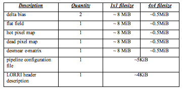 Table 9-14
Table 9-14 9.3.13 Memory Required ~ 100 MiB 9.3.14 Temporary File System Space Needed None 9.3.15 Predicted Size of Output File(s)
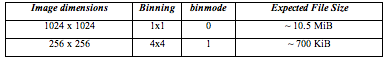 Table 9-15
Table 9-15 9.3.16 Predicted Execution time Less than 30 seconds per image. 9.3.17 Contact/Support Person(s) Raw data support: Howard Taylor, John Hayes, and Hal Weaver Calibrated data support: Howard Taylor and Hal Weaver 9.3.18 Maintenance Schedule (Code/Data Updates, Documentation) As in-flight calibration data are collected and analyzed, certain aspects of the calibration pipeline will require updates, either in the form of updated reference files, or updated code for bug fixes or future improvements. 9.4 References A. F. Cheng, H. A. Weaver, S. J. Conard, M. F. Morgan, O. Barnouin-Jha, J. D. Boldt, K. A. Cooper, E. H. Darlington, M. P. Grey, J. R. Hayes, K. E. Kosakowski, T. Magee1 E. Rossano, D. Sampath, C. Schlemm, H. W. Taylor, "LONG-RANGE RECONNAISSANCE IMAGER ON NEW HORIZONS", in Space Science Review, in press(2007) S. Conard, F. Azad, J. Boldt, A. Cheng, K. Cooper, E. Darlington, M. Grey, J. Hayes, P. Hogue, K. Kosakowski, T. Magee, M. Morgan, E. Rossano, D. Sampath, C. Schlemm, and H. Weaver, "Design and fabrication of the New Horizons Long-Range Reconnaissance Imager," in Astrobiology and Planetary Missions, G. R. Gladstone, ed., Proc. SPIE 5906, 2005. F. Morgan, S.J. Conard, H.A. Weaver, O. Barnouin-Jha, A.F. Cheng, H.W. Taylor, K.A. Cooper, R.H. Barkhouser, R. Boucarut, E.H. Darlington, M.P. Grey, I. Kuznetsov, T.J. Madison, M.A. Quijada, D.J. Sahnow, and J.M. Stock, "Calibration of the New Horizons Long-Range Reconnaissance Imager," in Astrobiology and Planetary Missions, G. R. Gladstone, ed., Proc SPIE 5906, 2005. 10. MVIC INSTRUMENT DESCRIPTION: 10.1 Overview The Ralph instrument consists of two sets of focal planes: MVIC a visible, near-IR imager and LEISA, a short-wave IR spectral imager. This document only relates to the MVIC (Multispectral Visible Imaging Camera) part of the Ralph instrument. The LEISA pipeline is described in a different document (New Horizons SOC to Instrument Pipeline ICD LEISA Edition). There are 7 separate CCD arrays in the MVIC focal plane. The MVIC telemetry is communicated via a low-speed interface and the imaging data uses a high-speed interface.
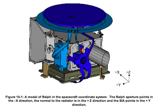 Figure 10-1 shows a model of Ralph in the spacecraft coordinate
system. The MVIC detector package is the light blue box on the +Y
face of the instrument.
Data recorded on New Horizons is sent to the ground via the Deep Space
Network. From there the data is sent to the Mission Operations Center
(MOC) at the Applied Physics Laboratory (APL). The Science Operations
Center (SOC) retrieves new data from the MOC daily. The data is in a
raw form (packetized). The Level 1 and 2 software pipelines convert
the data from these raw packets into FITS (Flexible Image Transport)
files with scientifically useful and calibrated data. The Level 1
processing sorts the packets into images (in the case of MVIC) with
useful header keywords. These keywords include the mode or filter of
the observation, timing information and basic pointing information of
the instrument boresight. The Level 1 processing also adds relevant
housekeeping telemetry (temperatures, voltages, etc.) in a binary
table as an extension to the FITS file. The Level 2 processing
performs the basic scientific calibration.
Before we get into a description of the MVIC calibration, we will
describe the image formats for each of the CCD arrays that comprise
MVIC. There are 8 detectors in the Ralph instrument. Seven of those
are part of MVIC (the yellow and blue ones). The boresight information
in the figure is from ground-testing and will change in the future.
Figure 10-1 shows a model of Ralph in the spacecraft coordinate
system. The MVIC detector package is the light blue box on the +Y
face of the instrument.
Data recorded on New Horizons is sent to the ground via the Deep Space
Network. From there the data is sent to the Mission Operations Center
(MOC) at the Applied Physics Laboratory (APL). The Science Operations
Center (SOC) retrieves new data from the MOC daily. The data is in a
raw form (packetized). The Level 1 and 2 software pipelines convert
the data from these raw packets into FITS (Flexible Image Transport)
files with scientifically useful and calibrated data. The Level 1
processing sorts the packets into images (in the case of MVIC) with
useful header keywords. These keywords include the mode or filter of
the observation, timing information and basic pointing information of
the instrument boresight. The Level 1 processing also adds relevant
housekeeping telemetry (temperatures, voltages, etc.) in a binary
table as an extension to the FITS file. The Level 2 processing
performs the basic scientific calibration.
Before we get into a description of the MVIC calibration, we will
describe the image formats for each of the CCD arrays that comprise
MVIC. There are 8 detectors in the Ralph instrument. Seven of those
are part of MVIC (the yellow and blue ones). The boresight information
in the figure is from ground-testing and will change in the future.
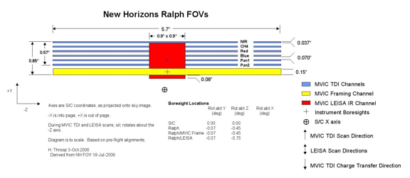 Figure 10-2
The "Pan Frame" array (yellow) has 5024x128 pixels. The first and
last 12 pixels in each row are not optically active. When observing
with the pan frame array, multiple images are recorded in each
observation. Correspondingly, we store these images together in one
FITS file. The first three letters of these files are "mpf" standing
for MVIC pan frame. The images are stored as an image cube
(3-dimensions). The first dimension is the column number, the second
dimension is the row number and the third dimension is the image
number within that observation.
The remaining 6 arrays are operated in a time-delay integration mode
(TDI). These arrays have 5024x32 pixels. The first and last 12 pixels
in each row are not optically active. To take an observation with the
TDI arrays, we scan the spacecraft and (typically) clock the charge
through each of the 32 rows at a rate that matches the spacecraft's
scan rate. Using this method we can build up arbitrarily long images
in the row direction. For the "Pan 1" and "Pan 2" (panchromatic --
unfilterred) detectors, the resulting FITS files are standard
2-dimensional images The first three letters of these files are either
"mp1" or "mp2" corresponding to MVIC pan 1 or MVIC pan 2. The color
arrays (NIR, CH4, Red and Blue) are operated together and they use a
time-delay integration to build up images. The data for each filter
is stored in separate FITS files.
In the table below the variable "Ni" stands for the number of images
in a pan frame observation. When we command a pan frame observation,
we always take multiple images. The "Nr" in the table is the number
or rows in an observations. This is determined by the length of time
that we are recording data and the rate that we clock the rows in TDI
mode.
Figure 10-2
The "Pan Frame" array (yellow) has 5024x128 pixels. The first and
last 12 pixels in each row are not optically active. When observing
with the pan frame array, multiple images are recorded in each
observation. Correspondingly, we store these images together in one
FITS file. The first three letters of these files are "mpf" standing
for MVIC pan frame. The images are stored as an image cube
(3-dimensions). The first dimension is the column number, the second
dimension is the row number and the third dimension is the image
number within that observation.
The remaining 6 arrays are operated in a time-delay integration mode
(TDI). These arrays have 5024x32 pixels. The first and last 12 pixels
in each row are not optically active. To take an observation with the
TDI arrays, we scan the spacecraft and (typically) clock the charge
through each of the 32 rows at a rate that matches the spacecraft's
scan rate. Using this method we can build up arbitrarily long images
in the row direction. For the "Pan 1" and "Pan 2" (panchromatic --
unfilterred) detectors, the resulting FITS files are standard
2-dimensional images The first three letters of these files are either
"mp1" or "mp2" corresponding to MVIC pan 1 or MVIC pan 2. The color
arrays (NIR, CH4, Red and Blue) are operated together and they use a
time-delay integration to build up images. The data for each filter
is stored in separate FITS files.
In the table below the variable "Ni" stands for the number of images
in a pan frame observation. When we command a pan frame observation,
we always take multiple images. The "Nr" in the table is the number
or rows in an observations. This is determined by the length of time
that we are recording data and the rate that we clock the rows in TDI
mode.
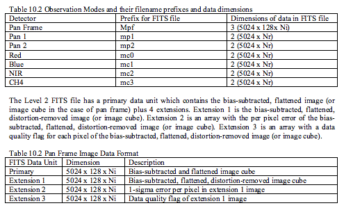 Table 10-2
Table 10-2 Observation Modes and their filename prefixes and data dimensions (top) Table 10-2 Pan Frame Image Data Format (bottom) The Level 2 FITS file has a primary data unit which contains the bias-subtracted, flattened image (or image cube in the case of pan frame) plus 4 extensions. Extension 1 is the bias-subtracted, flattened, distortion-removed image (or image cube). Extension 2 is an array with the per pixel error of the bias-subtracted, flattened, distortion-removed image (or image cube). Extension 3 is an array with a data quality flag for each pixel of the bias-subtracted, flattened, distortion-removed image (or image cube).
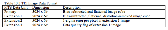 Table 10-3
Table 10-3 TDI Image Data Format 10.2 Level 1 Specifics 10.2.1 Data Format The Level 1 MVIC files will be FITS files. Details of the dimensions 10.of the FITS images and header keywords are given in the following 10.sections. 10.2.2 Data Sources (High/Low Speed, CCSDS, ITF) MVIC telemetry data are recorded using the low-speed interface and images are recorded with the high-speed interface. There are four Ralph-MVIC data formats: A. MVIC Panchromatic TDI (Time-Delay Integration) Format B. MVIC Panchromatic TDI Binning Format C. MVIC Color TDI Format D. MVIC Frame Format Note the distinction between "format" and "mode" is a hold over from the spacecraft to Ralph ICD where the LEISA component of Ralph has multiple modes for one format. The MVIC Panchromatic TDI format has two modes (either "Pan 1" or "Pan 2" indicating which detector was used). The MVIC Panchromatic TDI binning format is obsolete and is not being supported at this time. The remaining two formats each have only one mode. The columns in Table 10-4 list the MVIC ApIDs and their corresponding data types. For each data type there are two ApIDs, one for each C&DH (Command and Data Handling) system on the spacecraft.
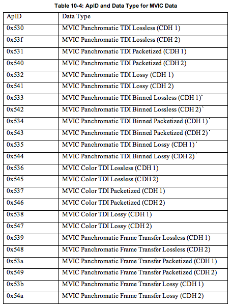 Table 10-4
Table 10-4: ApID and Data Type for MVIC Data *Note that the Panchromatic TDI Binned data is 3x1 binning in the cross-track direction with 2 out of 3 along-track lines discarded. Note there is not a different ApID for PAN1 and PAN2 observations. This information is stored in the low-speed housekeeping data (keyword MODE). This information is inserted into the FITS header of the Level 1 FITS file. A value of 3 means that the observation was taken with the "Pan 1" array and a value of 4 indicates the "Pan 2" array was used. For more information, see the Ralph Users Manual. The Pan Frame detector has 5024x128 pixels. The first and last 12 pixels in each row are not optically active. When observing with the pan frame array, multiple images are recorded in each observation. Correspondingly, we store these images together in one FITS file. The first three letters of these files are "mpf" standing for MVIC pan frame. The images are stored as an image cube (3-dimensions). The first dimension is the column number, the second dimension is the row number and the third dimension is the image number within that observation. The remaining 6 arrays are operated in a time-delay integration mode (TDI). These arrays have 5024x32 pixels. The first and last 12 pixels in each row are not optically active. To take an observation with the TDI arrays, we scan the spacecraft and (typically) clock the charge through each of the 32 rows at a rate that matches the spacecraft's scan rate. Using this method we can build up arbitrarily long images in the row direction. For the "Pan 1" and "Pan 2" (panchromatic -- unfilterred) detectors, the resulting FITS files are standard 2-dimensional images The first three letters of these files are either "mp1" or "mp2" corresponding to MVIC pan 1 or MVIC pan 2. The color arrays (NIR, CH4, Red and Blue) are operated together and they use a time-delay integration to build up images. The data for each filter is stored in separate FITS files. 10.2.3 Definition of an "Observation" For this ICD and as is consistent with the "New Horizons Spacecraft to PERSI/RALPH Interface Control Document", an "observation" is a coherent sequence of data-taking operations, with data reported over the high-speed telemetry interface conducted automatically after being initiated by telecommands from the C&DH system. The observation may end automatically, or may run until a telecommand ends it. All observations consist of one or more "frames." A "frame" is the amount of high-speed image data between returns of the +frame signal to the high state. All frames consist of a sequence of "words". A word is a pixel and is 12 bits in length. 10.2.4 Housekeeping Needed in Level 1 Files (for Calibration) There are some housekeeping values that we need to track for the health of MVIC and to assess the data quality. We need to monitor these keywords during Ralph observations. The Ralph telemetry will be sent each second during an MVIC observation and these keywords will be stored as a binary table in EXTENSION 1 of the Level 1 FITS file. They will be used to set the data quality flag if the value exceeds its yellow limit. The red and yellow limits in Table 10-1 are pre-launch limits and will be updated as needed.
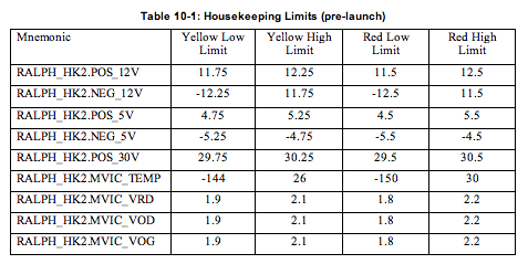 Table 10-1
Table 10-1: Housekeeping Limits (pre-launch) There are no additional raw science data requirements beyond those already specified. Ralph housekeeping data are stored in a binary table extension. Ralph specific keywords in the Level 1 file are given in the following Table. Keyword Description MET510 the MET of the Ralph 0x510 packet that marks the start of an observation TRUE510 Is the 0x510 real or assumed from a gap? RALPHEXP RALPH exposure time (s) MODE Instrument mode SIDE Instrument HW side FILTER CCD filter color, Only in MVIC Color FITS files PANCCD Pan CCD used (1 or 2), Only in MVIC Panchromatic TDI FITS files For the MVIC pan frame data, the standard keywords describing the pointing and mid-exposure time are repeated for each image in the image cube. 10.3 Level 2 Specifics 10.3.1 Algorithm for Pipeline There are five processing steps applied to the Level 1 MVIC data to 10.produce the Level 2 output: 7. Remove bias and flat-field pattern 8. Correct for a geometric distortion 9. Convert from DN to physical units 10. Calculate error for each pixel and construct the error array in a new extension 11. Construct data quality extension. Note there will not be any correction for scattered light (at least initially) in the Level 2 products. A complete assessment of the scattered light field will be made in flight, and corrections will be implemented if necessary. Also, there is no correction for cosmic rays in the Level 2 product. We do not apply the Level 2 calibrations to the non-optically active pixels of the detector to maintain our high-speed header data which is encoded in some of these pixels. 10.3.1.1 Remove bias and flat-field pattern First, the removal of the bias level and flat-field pattern for the framing array will be discussed, and then we will address modifications for the TDI modes. For the "Pan Frame" data, we use the shielded pixels on both sides of the array to compute the row-by-row bias. For column numbers 12 to 2511 (the active area on the left half of the chip), the bias is the median of pixels in columns 2 to 11 (inclusive and zero-based). Similarly, the bias for pixels from column numbers 2512 to 5011 (the active area on the right half of the chip) comes from the shielded pixels in columns 5012 to 5021 (inclusive and zero-based). We do not include the pixels closest to the edge of the array as they contain the high-speed header information. For the TDI mode, only pixels on one side of the image would be usable as bias level. The others are used for charge injection and do not represent the bias level. However, if we only use pixels from one side of the array we do not get a good model of the bias level. Instead we assume a fixed value of 24 DN for the bias level for all TDI arrays. The correction for the bias level and flat-field pattern are described here. Let B be the bias level, R is the raw image, and F is the normalized flat-field image: We calculate the corrected image, R_f in Equation 10-1.
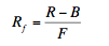 Equation 10-1
The name of the flat field file used will be stored in the header keyword FLAT. The naming convention for the flats will be unique. Each file name will contain the name of the array as well as the date (i.e. "flat_mvic_pan1_20050612.fits" or "dark_mvic_colorBlue_20050612.fits"). For our purposes, the dark current is expected to be negligible. For the TDI exposures, the flat field image is one-dimensional since each pixel in a given column is clocked through all 32 rows before being read out. This one-dimensional flat field has the dimensions of a single row in the TDI image. Instead of dividing the TDI image by a two-dimensional normalized flat, we will be dividing each row by the normalized (1-dimensional) flat. There will be 6 different flat-field one-dimensional arrays: 4 color and 2 panchromatic. There will only be one 2-D flat field image (for the framing array). The function that constructs the flattened, bias-subtracted image (Eq. 2) is called mvic_flatten. The function will determine what imaging mode was used (pan1, pan frame, etc), use the appropriate median flat field image, and produce an image with the bias subtracted, and flat field pattern removed. This image (or image cube, in the case of the pan frame detector) is stored in the primary data unit (PDU) of the Level 2 FITS file. 10.3.1.2 Geometric Correction Once again we will start with a discussion of the correction as applied to the framing array and then expand to describe the procedure for the TDI arrays. There are two sources of geometric distortion. The first is instrumental. This is the distortion due to optical effects in the instrument. The second source of distortion is motion distortion. This second source only affects TDI observations and is caused by the cross-track drift of the boresight within the deadband during the scan. For the following discussion, we define the following variables: N = number of images included in the analysis i = 0, ..., N = index running over the number of images p, q, ..., n = number of correlated star pairs identified for each image j = index running over all correlated stars in image i. e.g., if i = 0, j runs from 0 to p C_ji = column number of jth star in image i R_ji = row number of jth star in image i xi_ji^c = xi -coordinate of the catalog star correlated with the jth star in image i eta_ji^c = eta-coordinate of the catalog star correlated with the jth star in image i m_c, m_r = plate scales in column and row directions theta_i = FOV rotation of ith image, and is the angle measured in a counter-clockwise sense from the row-direction of the image to the positive eta-axis. n_c, n_r = number of columns and rows in the instrument CCD For image i, the transformation from column and row coordinates (C_ji, R_ji) to the tangent-plane coordinates (xi_ ji, eta_ji) is made using Equation 10-2, where C_ji' = C_ji - n_c/2 and R_ji' = R_ji - n_r/2, and ai
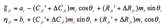 Equation 10-2
and bi are constants. The center of the FOV maps onto xi = a_i and eta = b_i. Delta(C_ji) and delta(R_ji) are perturbations about C_ji and R_ji that account for instrument distortion. If they are zero, and exact values of all other parameters in Equation (1) are known, then the xi_ji and eta_ji are equal to the catalog values xi_jic and eta_ji^c. delta(C_ji) and Delta(R_ji) are each modeled as a series of orthogonal polynomials: we use Legendre Polynomials, and we introduce the following normalization to scale C_ji' and R_ji' to the -1 to 1 range required Equation 10-3.
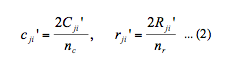 Equation 10-3
We adopt a fifth order Legendre polynomial model for the distortion model. This is the general kth-order bivariate polynomials. For our case k=5. Equation 10-4, where the vpq and wpq are unitless constants included
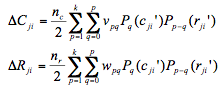 Equation 10-4
as free parameters in the least squares algorithm. Note that no zero-order terms are present (p > 1) since they are already represented by the offsets ai and bi in Equations (2). The number of terms in each polynomial is Equation 10-5.
 Equation 10-5
The vpq and wpq do not depend on i and j and there are a total of 2N_P of them, regardless of the number of stars and images. Also included in the list of free parameters for the least squares fit are the two plate scales (m_c and m_r), the N rotations (theta_i), and the 2N column and row offsets (a_i and b_i). The total number of free parameters is therefore M = 2 + 3N + 2N_P. The columns in Table 10-6 define the fitted parameters to 10 images that were used to define the distortion model.
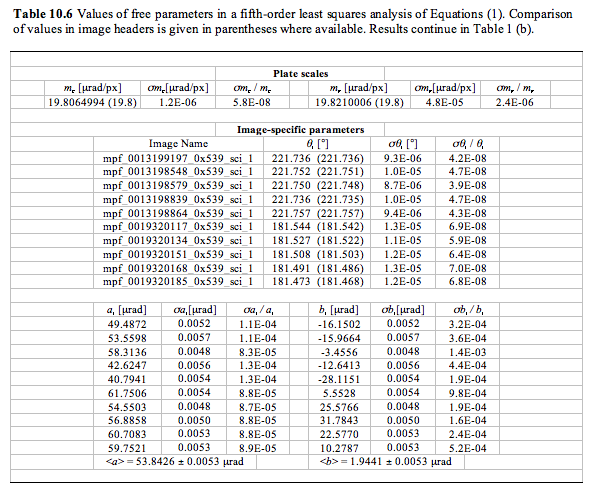 Table 10-6a
Table 10-6a Values of free parameters in a fifth-order least squares analysis of Equations (1). Comparison of values in image headers is given in parentheses where available. Results continue in Table 10-6b.
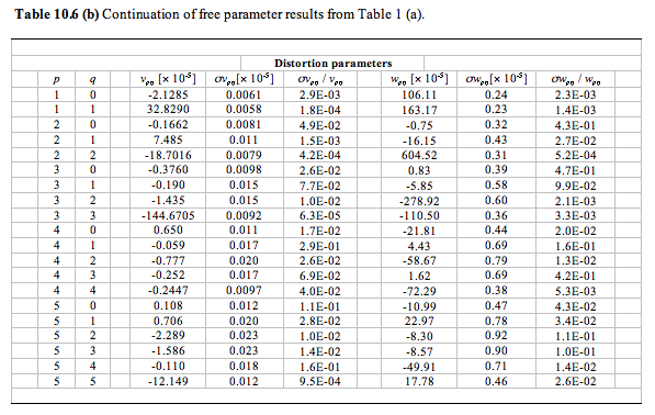 Table 10-6b
Table 10-6b Continuation of free parameter results from Table 10-6a. The standard deviation of the residuals is less than 0.1 pixel. The maximum distortion at the edge of the field (near column numbers 12 and 5000 is about 2.5 pixels. The navigation team would not like the image pixels remapped. For this reason, we will retain the image with the bias subtracted and flat field removed but without the geometric distortion correction and store this image in the primary data unit. This flattened, distortion-corrected image will be the first extension in the level two product. For the TDI images, we need to also correct the flattened image for motion distortion in the cross-track and along-track directions. The C-Kernel provides the spacecraft pointing information. The spacecraft scan can be oriented in any direction in space. From the C-Kernel, we get the pointing at the beginning and end of the scan and construct a line between those two points. This is our nominal scan path. Deviations from the linear path are the motion distortion. At the mid-exposure time for each pixel, we query the C-Kernel for the spacecraft pointing and compare that to our nominal scan path. We determine the cross-track and along-track errors from the nominal scan path and bilinearly interpolate the pixels in that row to correct for the motion distortion at the mid-exposure time of the row. We only correct for both the cross-track and along-track motion distortions. 10.3.1.3 Conversion to Physical Units We are using the same standard method as used by the LORRI instrument for conversion to physical units. In order to determine the conversion to physical units, we need to know the spectral type of the target.. We have determined the conversion factor for 4 different spectral types: Pluto, Charon, Jupiter, Solar and Pholus. The absolute calibration is given by a keyword (i. e., RPLUTO) in the header of the Level 2 file that allows the user to convert a count rate ("C/TEXP" in DN/s/pixel, where "C" is the flat-fielded signal in a pixel and "TEXP" is the exposure time) for a resolved source into a radiance value ("I" in ergs/cm^2/s/sr/Angstroms) at MVIC's pivot wavelength (specified by the FITS keyword PIVOT; see below), assuming that the spectrum of the target is identical to the globally-averaged spectrum of Pluto. The relevant formula is: I = C/TEXP/RPLUTO The keyword RPHOLUS allows the conversion of the count rate for a resolved source into a radiance value at the pivot wavelength assuming that the target has a spectral distribution identical to that of the centaur object 5145 Pholus, which may be a good analog for the reddest regions on Pluto: I = C/TEXP/RPHOLUS Similarly, the keywords RSOLAR, RJUPITER and RCHARON provide the conversion factors for resolved targets with Solar-, Jupiter- or Charon-like spectra. Table 10-7 gives the values of the multiplicative factor (RSOLAR, RJUPITER...) for resolved objects.
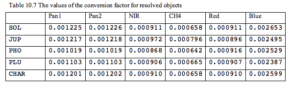 Table 10-7
Table 10-7 The values of the conversion factor for resolved objects. The pivot wavelength (PIVOT) is given by Equation 6, where "P" is the MVIC system quantum efficiency (i.e., fraction of photons detected) at wavelength "lambda". The pivot wavelength is passband specific and is stored in the FITS file header.
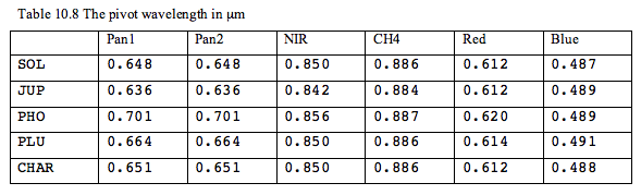 Table 10-8
Table 10-8 The pivot wavelength in microns. For unresolved sources (e.g., stars), the calibrated flux (also called "irradiance") at the pivot wavelength can be determined using keywords that are defined analogously to the photometry keywords discussed above for resolved sources. In the case of a source having a spectral distribution identical to that of a globally-averaged Pluto spectrum, the observed count rate integrated over the MVIC PSF ("CINT/TEXP" in DN/s, where CINT is the total number of flat-field corrected counts integrated over the image and "TEXP" is the exposure time) can be related to the flux ("F" in ergs/cm^2/s/Angstroms) by: F = CINT/TEXP/PPLUTO Similarly, the flux at the pivot wavelength for a target having the same spectral distribution as Charon (PCHARON), the sun (PSOLAR), and Pholus (PPHOLUS) are given in the FITS header.
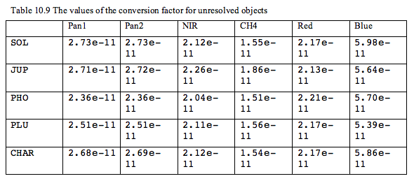 Table 10-9
Table 10-9 The values of the conversion factor for unresolved objects 10.3.1.4 Error Propagation The standard deviation of each pixel will be calculated and the resulting 2-D array of errors will be put into extension 2 of the FITS file. The gain, g, and the DN value of each pixel of the distortion-removed flattened image (extension 1 in the FITS file) will be used to determine the photon noise. The photon noise and the read noise, RN, will be used to calculate the standard deviation per pixel in DN. The error equation, Equation 10-7.
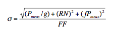 Equation 10-7
The gain (58.6 electrons per DN) and read noise (30 electrons) values used to calculate the standard deviation will be entered in the file header with the keywords GAIN and READNOI. We will also include the error propagation due to uncertainty in the flat field pattern. Other sources of error such as the uncertainty in the bias level are not included. (XXcheck the error equation not that I will be doing it for the distortion corrected image which already has the flat field pattern removed). 10.3.1.5 Data Quality Flags The data quality flags will be set to a non-zero value if there is a problem with the data and zero if the data is fine. Below is a preliminary list of the factors that will cause the data quality flag to be set to its appropriate value. Quality Flag Value Description 0 Good pixel 1 Housekeeping keyword out of yellow limits, see Table 10-1. 2 Defect in one of the reference calibration files 4 Permanent CCD defect (e.g., dead pixel) 8 DN level in non-linear regime of detector 16 Zero-value pixel 32 Bad pixel not in any of above categories -1 Missing data If a housekeeping keyword exceeds it's yellow limit at any time during the exposure the data quality flag for all the pixels in the image are set to 1. 10.3.2 Dataflow Block Diagram (to do - add distortion correction to tree) Here is a diagram that shows how the data flows through the different IDL procedures and functions that comprise the Level 2 pipeline. ; mvicL2_pipeline ; | ; --mvic_level2_pipeline ; | ; --mvic_flatten ; | | ; | --pantdi_flatten ; | | | ; | | --pantdi_readflat ; | | | ; | | --tdi_flatten_core ; | | ; | --mcl_flatten ; | | | ; | | --mcl_readflat ; | | | ; | | --tdi_flatten_core ; | | ; | --panfra_flatten ; | ; --mvic_geo ; | ; --mvic_dq ; | | ; | --pantdi_dq ; | | ; | --check_pixels ; | | ; | --pantdi_hk_check ; | | | ; | | --setUpAndScaleHK ; | | | ; | | --scaleRawRalphTelemetry ; | | | ; | | --conversionCoefsForMVIChk.pro ; | --panfra_dq ; | | ; | --panfra_check_pixels ; | ; | ; --mvic_err ; | ; --pantdi_err ; | | ; | --pantdi_readflat ; | ; --mcl_err ; | | ; | --mcl_readflat ; | ; --panfra_err 10.3.3 Data Format All of the MVIC Level 2 FITS files have a primary data unit and four extensions. In the primary data unit, the bias-subtracted, flattened data is stored. The first extension has the bias-subtracted, flattened, distortion-removed data. The second extension has the error array for the bias-subtracted, flattened, distortion-removed data. The third extension has the data quality array for the bias-subtracted, flattened, distortion-removed data. The fourth extension is the binary table containing the instrument housekeeping. The image data for the TDI observations is stored in a a two-dimensional array. The number of columns in the array is always 5024. The number of rows in the array depends on the duration of the observation and the scan rate. The image data for the pan frame observations is stored in a three-dimensional array (an image cube). The number of columns is always 5024, the number of rows is always 128. 10.3.4 Scientific Units We will be using cgs units for the Level 2 output. The flux per pixel will have the units of ergs/s/cm2/Angstrom. 10.3.5 Additional FITS and PDS Keywords Added Additional FITS keywords added to the Level 2 product include: SOCL2VER= '1.0 ' /Version of Level 2 software PIXSIZE = 13.0000 /Pixel size in microns PIXFOV = 19.8000 /Single pixel field of view in microradians READNOI = 30.0000 /Readnoise in Electrons GAIN = 58.6000 /Gain in Electrons/DN CALDIR = 'cal/ ' /Directory for calibration files PPHOLUS = /(DN/s)/(erg/cm^2/s), Pholus spectrum PPLUTO = /(DN/s)/(erg/cm^2/s), Pluto spectrum PSOLAR = /(DN/s)/(erg/cm^2/s), Solar spectrum RPHOLUS = /(DN/s/pix)/(erg/cm^2/s/sr), Pholus spectrum RPLUTO = /(DN/s/pix)/(erg/cm^2/s/sr), Pluto spectrum RSOLAR = /(DN/s/pix)/(erg/cm^2/s/sr), Solar spectrum PIVOT = /cm, pivot wavelength The values of the radiometric keywords are source dependent as discussed above. 10.3.6 Extra FITS Extensions() and Their Definitions There are four extra FITS extensions. The first three have been described in detail previously (the distortion-removed image file, the error array and the data quality flag array). The fourth extension is the binary table with the housekeeping data. This data is simply passed along from the Level 1 file without modification. 10.3.7 Hardware/OS Development Platform The Level 2 software will be developed on a PowerBook G4 running Mac OS X version 10.3.4. Future Migration will be backwards compatible. 10.3.8 Language(s) Used The MVIC Level 2 software will be written using IDL. 10.3.9 Third Party Libraries Required The code will require the "IDL Astronomy User's Library". It is available from http://idlastro.gsfc.nasa.gov/homepage.html. 10.3.10 Calibration Files Needed (with Quantities) The following calibration files will be used. - Flat field images for each array - Bad pixel files for each array - File with the acceptable levels of the housekeeping keywords that we are monitoring There will probably be multiple generations of each over time during the mission. These files will be archived with the observations ] 10.3.11 Memory Required TBD 10.3.12 Temporary File System Space Needed None. 10.3.13 Predicted Size of Output File(s) The output files will be approximately twice as large as the input files since we are adding the multiple extensions, but not propogating the housekeeping. 10.3.14 Predicted Execution time TBD 10.3.15 Contact/Support Person(s) Cathy Olkin Dennis Reuter Leslie Young 10.3.16 Maintenance Schedule (Code/Data Updates, Documentation) The code will be updated on the schedule mandated by the mission. The current plan is to do code maintenance after the Instrument Calibration (on the ground), after Integration and Test (on the ground), after Commissioning, and after the Jupiter Encounter. Calibration files will be updated throughout the mission as necessary. Necessary criteria include new calibration information (such as new flat-field observations or a new geometric distortion correction) such as might be available after an annual checkout. 11. PEPSSI INSTRUMENT DESCRIPTION 11.1 Overview 11.1.1 PEPSSI Investigation PEPSSI (Pluto Energetic Particles Spectrometer Science Investigation) is a hockey-puck-size, time-of-flight (TOF) spectrometer that measures ions and electrons over a broad range of energies and pitch angles. Particle composition and energy spectra be measured for H to Fe from ~15 keV/nucleon to 1 MeV/nucleon and for electrons from 15 keV to 700 keV. The PEPSSI instrument traces its heritage back to the MESSENGER Energetic Particle Sensor (EPS) instrument. EPS/PEPSSI was developed with the support of a NASA Planetary Instrument Definition and Development (PIDDP) grant aimed at designing a low-mass, low-power sensor that can measure energetic pickup ions produced near planets and comets (Andrews et al., 1998; McNutt et al., 1996). The overall PEPSSI instrument weighs 1.5 kg and uses maximum power of 1.4 W. Figure 2 shows the placement of PEPSSI on the spacecraft and the PEPSSI fields-of-view (FOV). The science goals of the PEPSSI instrument are: 1. Determine the escape rate of Pluto's atmosphere 2. Measure the interaction of the solar wind with Pluto's ionosphere 3. Determine the source and nature of energetic particles found near Pluto 11.1.2 PEPSSI Sensor Description PEPSSI is a compact particle telescope with a time-of-flight (TOF) section and a solid-state detector (SSD) array (see Figure 3). A mechanical collimator defines the acceptance angles for the incoming ions and electrons. A cutaway view of the assembly is shown in Figure 4. The TOF section is axially symmetric; entrance and exit apertures are 6 mm wide with an azimuthal opening angle of 160degrees. The entry and exit apertures are covered by thin (~7 microg/cm2) polyimide/aluminum and (~10 microg/cm^2) palladium/carbon foil mounted on high-transmittance stainless-steel grids, respectively. The foil thickness and composition is a compromise to minimize the energy threshold, secondary electron production, and scattering of particles in the foil while blocking UV from the direct Sun and Lyman-alpha background. PEPSSI measures the ion TOF using secondary electrons generated as the ion passes through the entrance and exit foils in the spectrometer. Total energy is measured by the SSD array. Each of the six SSDs has two pixels, three of the SSDs are dedicated for ion measurement. The other three have one pixel covered with ~1 microns Al absorber, to block low energy ions and permit measurements of electrons. The fan-like collimator together with the internal geometry defines the acceptance angles. The FOV is 160degrees by 12degrees with six angular sectors of 25degrees each; the total geometric factor is ~0.15 cm^2sr. As an ion passes through the sensor, it is first accelerated by the potential of ~3 kV on the front foil prior to hitting it. The ion generates secondary electrons at the foils, which are then electrostatically steered to well-defined separate regions on a single micro channel plate (MCP), providing "start" and "stop" signals for the TOF measurements (from 1 ns to 320 ns). The segmented MCP anode, with one start segment for each of the six angular entrance segments, allows determination of the direction of travel even for lower-energy ions that do not give an SSD signal above threshold. The combination of measured energy and TOF provides unique particle identification by mass and particle energy in the range: for protons from 15 keV to 1 MeV; for heavy (CNO) ions from 80 keV to 1 MeV. Lower-energy (>3 keV) ion fluxes are measured by TOF and pulse-height analysis (PHA) of the signal they produce in the MCP, providing particle identification and velocity spectra at these energies as well. Molecular ions, expected from Pluto's atmosphere, will break up in the foil prior to their full detection, but will be detected as high-mass events. Internal event classification electronics determine the mass and produce an eight-point energy spectrum for each of four species for six arrival directions. Energetic electrons are measured simultaneously in the dedicated electron pixels in the range from 20 to 700 keV. Only protons with energies > 300 keV (expected to be very rare at Pluto) can penetrate the absorbers on these pixels, and even those would be eliminated by on-board MCP coincidence requirements and ground comparisons with the simultaneously measured ion flux. 11.1.3 PEPSSI Electronics Description Extensive uses of miniaturization and custom electronic in the design allow PEPSSI to weigh less than 1.5 kg and consume less than 1.4 W. PEPSSI is made up of six modular 4"x4" slices. They consist of: 1) Energy board; 2) High Voltage Power Supply (HVPS); 3) TOF board; 4) Digital processing board; 5) Common event processor board; and 5) Low Voltage Power Supply (LVPS) board. See Figure 11-5 below which shows the exploded view of PEPSSI with each board labeled. A brief description of the functionality of each board is highlighted below. Energy board: The energy board is the interface between the SSDs and the signal conditioning electronics. It houses the sensor, MCP anodes, charge amplifiers, pulse shapers, etc. In addition, it also outputs the pulse signal from the 6 start anodes and 1 stop anode. HVPS board: The HVPS board contains the high voltage (HV) drive circuitry, HV transformer, and its control circuitry. It provides HV up to -2900 V for the sensor electrostatic lens and MCP bias. In addition, the HVPS also needs to provide bias voltage over the range of 0 to -200 V with <10 mV ripple. Digital processing board: The digital processing board provides valid event logic functions, which include channel enables, programmable coincidence window, event packet generation and rate counters for event statistics. It provides the logic to distinguish between electrons, ions and directionality. Common event processor board: This board contains PEPSSI's main processor (RTX2010RH), the Filed Programmable Gate Array (RT54SX72S), and various memory modules (SRAM, EEPROM, PROM). LVPS board: This board converts primary spacecraft power into multiple low voltage outputs used by PEPSSI. It provides highly efficient power conversion into two digitals (+5, +2.5V) and four analogs (+5, -5, +15, and -15) outputs. 11.2 Introduction to PEPSSI Data The PEPSSI instrument can operate in two modes: Normal and Diagnostic. On the spacecraft, each event generates a PHA record. This record is classified by event type: Electron, High-Energy Ion (or "Hi-Ion" or "Triple"), or low-energy ion (or "Low-Ion," "Double," or "TOF-only"). In diagnostic mode, events are not classified; alternatively, all events are "diagnostic events". Events of a given type are further classified into "Rate Boxes" by their energy and/or time of flight (TOF). Thus each event has a type, a rate box, and a detector in which it occurred. Instead of detector number, we will often use arrival direction (or sector) since there is a one to one relation between them (see figure 6). A six character string is used to specify each possible classification (or Rate) of an event. The construction of this string is (type)(rate box)S(arrival sector). The arrival sector numbering is shown in figure 6. The "type" string is: B - Hi-Ions (possesses Energy and TOF) R - Electrons (energy only, no TOF) L - Low-Ions (TOF-only, no-energy). For High Energy Ions, the "Rate Boxes" are determined by areas in the TOF vs Energy plain (see figure 7). These correspond to different particle species and different energies. For Electrons, the "Rate Boxes" are determined by energy ranges. For Low Energy Ions, the "Rate Boxes" are determined by TOF ranges and by which heavy ion discriminators fired. The definition of Low-Ion "Rate Boxes" has been changed for the post-Jupiter phases of the mission. Note that because of the way the PEPSSI electronics work, frequently the arrival sector is unknown or uncertain for the Low-Ion measurements. Some examples: B02S04 - High-Energy Rate Box #2, arriving from the sector 4 direction. Protons with deposited energy in channels 95-169 , in analog-to-digital units(ADUs). L06S03 - Low-Ions Rate # 6 arriving from the sector 3 direction. Ions with TOF indices from 45-79 ADUs and for which the heavy ion discriminator H0 fired but H1 didn't. R00S05 - The 0th electron rate, arriving from the sector 5 direction. Electrons with Energy channels in the range 720-1023 ADUs . There are two counters for each Rate that are incremented whenever a corresponding event occurs. The N2 counter is accumulated for a certain time interval (usually 15, 30, or 60 seconds), then recorded and zeroed. The N1 counter is accumulated for some multiple of the N2 interval (usually 10 minutes), then recorded and zeroed. A certain number of PHA events are kept according to a complex priority scheme and telemetered along with the Rate data. (Note: if the multi-hit, i.e. anti-coincidence, flag is set for an event, the event is not counted. This is programmable, but the "don't count multi-hit events" rule was true outside of Bad Time Intervals for the whole Jupiter phase). Various housekeeping and status data and certain global hardware and software counters are also present in the data at Levels 1 and 2. PEPSSI Level 1 and PEPSSI Pre-Level 2 data are internal formats that are not used outside the SOC. PEPSSI Level 2 data represents, with 3 exceptions, the raw data taken from the spacecraft telemetry. It has merely been reformatted for ease of use. No data has been added, removed or altered with the following 3 exceptions: a. Instrument Status information has been calibrated to physical units where applicable (see discussion in section 1.2.1.7 below). b. For clarification, a "DT" column has been added to the Rate tables to indicate the integration time over which the count data was accumulated. This information is not available in the spacecraft telemetry and must be calculated from the available timestamps. This "DT" value may be inaccurate during Bad Time Intervals (BTIs), see below. c. For ease of use, we have added a column giving the deduced "Rate Box" of High-Ion PHA and Electron PHA events to the Level 2 PHA data. While this can, in principle, be calculated from the raw Level 2 quantities and the instrument configuration files available in the calibration file section of the PDS archive, the procedure is complex enough that we have found it convenient to perform this calculation in advance and include the information in the Level 2 files. PEPSSI Level 3 data presents the data in a format that should be convenient for scientific analysis. All of the calibration parameters needed to convert Level 2 data to Level 3 data are present in the headers of the Level 3 data files. The formula's used to calculate the calibrated quantities are also present in the Level 3 headers. Rate data is presented in physical flux units with uncertainties as well as counts per second. PHA data is presented with calibrated TOF and deposited energy. Further calibrated incident energies are given for assumed ion species. Only PHA data telemetered with the N2 rates is present in Level 3 as discussed below. There are also some "quick look" PHA images and Rate spectrograms in the Level 3 data to allow for a simple overview of one day's observations. No "multi-hit" events are present in Level 3 PHA data. No diagnostic mode data is present in the Level 3 data. BTI data is present in the Level 3 data but should be ignored. Level 3 data for the "Launch" phase is present for quick-look purposes, but, apart from the deposited energy calibration (which is well known), the calibrations are performed with dummy values, as will be evident from examination of the header information. Note: End users of PEPSSI data (i.e. those outside the instrument team and the SOC) will probably not find much useful information in the Level 1 and Pre-Level 2 documentation which follows and are when reading this document are encouraged to skip directly to section 11.4.3, Level 2 Data. 11.3 Level 1 Specifics The SOC Level 1 data product is a FITS format data file and all data is contained in FITS extension Header Data Units (HDUs). Each HDU contains a PEPSSI science data telemetry block which is described in depth in the PEPSSI Flight Software Specification. Level 1 files are not present in the PDS archive. They are: File Type HDU Type N1 Primary HDU: High Priority Telemetry Block Extension 1: PHA Telemetry Block Extension 2: Status Telemetry Block N2 Primary HDU: Medium Priority Telemetry Block Extension 1: PHA Telemetry Block Extension 2: Status Telemetry Block N3 Primary HDU: Low Priority PHA Telemetry Block 11.3.1 Data Sources (High/Low Speed, CCSDS, ITF) PEPSSI is low-speed only. Data will be from CCSDS packets. 11.3.2 Definition of an "Observation" PEPSSI doesn't make specific "Observations". 11.3.3 Header with Keywords 11.3.4 Spacecraft Housekeeping Needed in Level 1 Files (for Calibration) Spacecraft attitude is necessary to calculate PEPSSI pointing in the ecliptic coordinate system, and with respect to Jupiter, Pluto, and Charon. An accuracy of 1 degree is adequate. 11.3.5 Raw Science Data and/or Housekeeping Requirements No special requirements 11.4 Level 2 Specifics 11.4.1 Algorithm for Pipeline 11.4.1.1 IDL L1 to Pre-L2 step The PEPSSI pipeline conversion from Level 1 (L1) to Level 2 (L2) data has two steps. The first uses an IDL program to rearrange the Raw L1 data into single-rowed vector-valued FITS tables. These "Pre-L2" files are temporary and not in the final PDS archive. Multiple Pre-L2 files will be combined in the next processing step into final L2 files; see section 11.3.1.2 below. The base routine PEPSSI_LEVEL2_PIPELINE reads from the input file the following variables: Filein dir_cal temp_dir status_file fileout and generates in the output files one of more of the corresponding HDUs N1 N1_STATUS N2 N2_STATUS D_N1 D_N2 PHA_ELECTRON PHA_LOW_ION PHA_HIGH_ION PHA_DIAG STATUS Decoding of the level 1 data stream follows two steps: first blocks are read into the 7 structures: N1 = { $ met:lonarr(blockcnt), $ high_ions:lonarr(6,19,blockcnt), $ electrons:lonarr(3,3,blockcnt), $ low_ions:lonarr(7,16,blockcnt), $ rates:lonarr(32,blockcnt), $ housekeeping:fltarr(33,blockcnt) } N2 = { $ met:lonarr(blockcnt), $ high_ions:lonarr(6,19,blockcnt), $ electrons:lonarr(3,3,blockcnt), $ low_ions:lonarr(7,8,blockcnt), $ rates:lonarr(24,blockcnt) } PHA_ELECTRON={ $ met:lonarr(ele_cnt) , $ energy:fltarr(ele_cnt) , $ multi:intarr(ele_cnt) , $ chann:intarr(ele_cnt) } PHA_LOW_ION={ $ met:lonarr(low_cnt) , $ tof:fltarr(low_cnt) , $ heavy1:intarr(low_cnt) , $ heavy0:intarr(low_cnt) , $ startseg:intarr(low_cnt) } PHA_HIGH_ION={ $ met:lonarr(hig_cnt) , $ energy:fltarr(hig_cnt) , $ tof:fltarr(hig_cnt) , $ multi:intarr(hig_cnt) , $ heavy1:intarr(hig_cnt) , $ heavy2:intarr(hig_cnt) , $ chann:intarr(hig_cnt) , $ startseg:intarr(hig_cnt) } PHA_DIAG={ $ met:lonarr(dia_cnt) , $ energy:fltarr(dia_cnt) , $ tof:fltarr(dia_cnt) , $ start:intarr(dia_cnt) , $ stop:intarr(dia_cnt) , $ fired:intarr(dia_cnt) , $ multi:intarr(dia_cnt) , $ heavy1:intarr(dia_cnt) , $ heavy0:intarr(dia_cnt) , $ chann:intarr(dia_cnt) , $ startseg:intarr(dia_cnt) } STATUS = { $ MET:lonarr(nsta), $ STATINT:lonarr(nsta), $ MACBLCKS:lonarr(nsta), $ TLMVOL:lonarr(nsta), $ WTCHADDR:lonarr(nsta), $ WTCHMEM:bytarr(nsta), $ WTCHDATA:lonarr(nsta), $ PEPSWVER:bytarr(nsta), $ ALARMID:bytarr(nsta), $ ALARMTYP:bytarr(nsta), $ ALARMCNT:bytarr(nsta), $ CMDEXEC:bytarr(nsta), $ CMDREJCT:bytarr(nsta), $ MACEXEC:bytarr(nsta), $ MACREJCT:bytarr(nsta), $ MACROID:bytarr(nsta), $ MACROLRN:bytarr(nsta), $ MONRESP:bytarr(nsta), $ WRITEENB:bytarr(nsta), $ HVPSCURR:fltarr(nsta), $ HVPSVOLT:fltarr(nsta), $ BIASCURR:fltarr(nsta), $ BIASVOLT:fltarr(nsta), $ PEPSTAT:lonarr(nsta), $ DVOLTP5:fltarr(nsta), $ AVOLTN5:fltarr(nsta), $ VOLTP2:fltarr(nsta), $ VOLTN5:fltarr(nsta), $ VOLTP15:fltarr(nsta), $ VOLTN15:fltarr(nsta), $ DCURRP5:fltarr(nsta), $ ACURRP5:fltarr(nsta), $ CURRP2:fltarr(nsta), $ CURRN5:fltarr(nsta), $ CURRP15:fltarr(nsta), $ CURRN15:fltarr(nsta), $ PRIMCURR:fltarr(nsta), $ LVPSTEMP:fltarr(nsta), $ ENGYTEMP:fltarr(nsta), $ HVPSTEMP:fltarr(nsta), $ ADDR12C:lonarr(nsta), $ RSLT12C:lonarr(nsta) $ } where blockcnt is the number of blocks present in the level 1 file (i.e. the number of sample periods), ele_cnt is the number of electron pha events, and similarly for low_cnt, hi_cnt, and dia_cnt. nsta is the number of sample periods for the status quantities. See the full L2 file description for the meaning of the status quantities. Example: n1.low_ions(3,4,6) corresponds to the number of time_of_flight only events (low_ions) coming from anode 3, 4th velocity bin, collected during the 6th time interval. 11.4.1.2 MIDL L1 to Pre-L2 step A Java program derived from the MIDL analysis program is used to convert the Pre-L2 files into L2 files. The L2 files contain exactly one day of data, except on days when new Rate Box definitions are loaded to the spacecraft in which case there will be a "before" file and an "after file"(these load-days are very rare). The DataConverter program essentially "flattens out" the Pre-L2 structure. In the L2 files, each row is a separate sampling period or PHA event (i.e. the blockcnt, hi_cnt, lo_cnt, etc. axis is now the row structure of the FITS binary table). Each "Rate Box" or hardware count is a separate column in the N1 or N2 FITS table. So, for example, each row of the N1 rates extension represents a separate sampling period (usually 600 seconds) and each column is a different rate, listed in alphabetical order by rate name, so the columns would be: ET, MET, B00S00, B00S01, ..., B18S05, C00D00, C01D01, ..., C23, C24, HK00, HK01, ...,HK34, J00, J01, ..., J06, L00S01, L00S02, ..., L15S05, L15SUnknown, R00S00, ..., R02S05 The meaning of the individual Rate Labels will be discussed below, or see the comments in the corresponding FITS header. As another example, the PHA_ELECTRON extension is another simple 2D table of values; each row represents a separate PHA event, the columns are: ET, MET, APID, Cross_Talk_Indicator, Electron_Channel, Raw_Energy 11.4.2 Dataflow Block Diagram
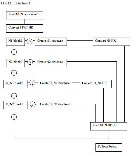 Figure 11-1a Dataflow Block Diagram, Part A
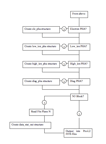 Figure 11-1b Dataflow Block Diagram, Part B
11.4.2.2 Pre-L2 to L2 processing
There is no data-flow diagram for Pre-L2 to L2 processing.
11.4.3 L2 Data Format
The contents of the in the L2 files are detailed in the following
sections. The ordering of the extensions is not guaranteed, programs
accessing the data should search for the desired extension by name (in
the EXTNAME keyword). There will always be only one extension of each
type (EXTNAME) and not all types will be present. An extension will
only be present if there is data of that type taken during the time
period covered by that file. Each file will contain exactly one
observing day worth of data (i.e. one UTC day from hour 0 -
23:59:59.999...). The Primary HDU contains no data, only informational
header keywords identifying mission info, observational start time,
and information about the file creation (date, software version,
etc.).
The available extensions are:
D_N1, D_N1_STATUS, D_N2, D_N2_STATUS, N1, N1_STATUS, N2, N2_STATUS,
PHA_DIAG, PHA_ELECTRON, PHA_LOW_ION, PHA_HIGH_ION
The different extensions are described below. For detailed
information such as the data-type of different columns see the FITS
header in the data file.
Extension names beginning with "D_" (and the PHA_DIAG extension)
represent data taken in diagnostic mode. Diagnostic data is taken for
purposes of calibration and understanding the instrument at a very low
level. Diagnostic data is complex and often taken under unusual
conditions. It is unlikely that the general user will be able to use
diagnostic data in any meaningful way. In diagnostic mode, a PHA
event is generated whenever any of the instrument detectors sees an
event. All events are counted except for those with the multi-hit
flag set (by default, the multi-hit setting can be changed). This
means that there are no "Low-Ion" events because, by definition, these
events are required to have no SSD fire, which is mutually exclusive
with the diagnostic mode requirement that every diagnostic event is
initiated with an SSD fire. Many of the columns will contain "fill
values" for certain types of events. The "Fill" values for invalid
Energy and TOF PHA data are: Energy - 1023 and TOF - 2047. In the
PHA_DIAG extension, what would normally be an electron event, for
instance, will have a Time of Flight value of 2047.
11.4.3.1 PHA_HIGH_ION
When an ion enters the PEPSSI detector, if it has enough energy, we
measure an Energy and a Time of Flight (TOF). Since we don't have
enough bandwidth to telemeter all of our events, we use a round robin
priority scheme to decide which PHA events to discard and which to
telemeter. All of the events are counted in the N1 and N2 Rate
data. The Rate data can be used to remove the priority group effects
(to a large extent) from the PHA data by weighting events by their
respective rates. See the L3 documentation below for more on
rate-weighting.
The PHA_HIGH_ION extension contains one row for each high energy ion
event that was not discarded by the priority scheme. The columns are:
ET Ephemeris Time (J2000)
MET Mission Elapsed Time
APID Which APID was this event telemetered in:
N1 - 0x691, N2 - 0x692, N3 - 0x693
Cross_Talk_Indicator Did more than one detector fire?
H0 Did Heavy Ion Descriminator 0 fire?
H1 Did Heavy Ion Descriminator 1 fire?
Ion_Channel Detector Channel (0-8)
Raw_Energy Energy deposited (ADU)
Raw_TOF Time of Flight (ADU)
Start_Anode Bits 0-5 are set if that start anode fired.
Notes on PHA High Ion data:
-IMPORTANT NOTE: The timing of a PHA event is not known to 1
second precision. The "time tag" of a PHA event only
represents the end time of the accumulation interval of the
Rate packet with which it was telemetered. So, in normal
operation, "N1 PHA" event arrival times are known only to the
nearest 10 minutes, N2 events to the nearest minute, and N3
events to within 2 hours. See discussion of Level 3 PHA data
for more details.
- Mission Elapsed Time starts about 19-JAN-2006-18:09:05.184.
See figure 6 for a diagram of the detector numbering. 9 of the 12
detectors are dedicated to Ions (the other 3 are dedicated to
electrons) and are configured accordingly.
- The H0 and H1 ion discriminators were found to be of limited usefulness.
Events with the Cross_Talk_Indicator value set are discarded from
the rate counters and are not usually used in analysis.
- Energy and TOF are given in raw "Analog to Digital Units" (ADU).
The Start Anode column consists of a single byte. The individual
bits 0-5 indicate whether the corresponding Start Anode (0-5)
registered an event. See figure 6 for start anode layout. Note
that, unfortunately, the numbering of the anodes is reversed from
the numbering of the incoming angle sectors.
- The electronics of the Start Anodes are such that, while a given
event may have a known TOF, the exact Start Anode information may be
uncertain or completely unknown. Thus, a valid event may show more
than one Start Anode, or none.
11.4.3.2 PHA_ELECTRON
The PHA_ELECTRON data is very similar to the PHA_HIGH_ION data except
that the TOF-related values aren't present since electrons aren't
detected by that part of the instrument (i.e. they only have solid
state detector (SSD)-related values:
ET Ephemeris Time (J2000)
MET Mission Elapsed Time
APID Which APID was this event telemetered in
Cross_Talk_Indicator Did more than one detector fire?
Electron_Channel Detector Channel (0-2)
Raw_Energy Energy deposited solid state detector (ADU)
Notes:
- Only Sectors 0, 2, and 5 have electron detectors (0,1, and 2,
respectively) associated with them.
See PHA_HIGH_ION notes for other relevant info.
11.4.3.3 PHA_LOW_ION
The PHA_LOW_ION events are from low energy ions that register in the
TOF part of the detector but do not trigger the SSDs. Hence "Low
Ions" have TOF data (and associated quantities like Start Anode) but
no Energy data:
ET Ephemeris Time (J2000)
MET Mission Elapsed Time
APID Which APID was this event telemetered in
H0 Did Heavy Ion Descriminator 0 fire?
H1 Did Heavy Ion Descriminator 1 fire?
Raw_TOF Time of Flight (ADU)
Start_Anode Bits 0-5 are set if that start anode fired.
See PHA_HIGH_ION notes for other relevant info.
11.4.3.4 PHA_DIAG
In diagnostic mode, the following columns are present:
ET Ephemeris Time (J2000)
MET Mission Elapsed Time
APID Which APID was this event telemetered in?
Cross_Talk_Indicator Did more than one detector fire?
Fired 0 - electron event 1 - ion event
H0 Did Heavy Ion Descriminator 0 fire?
H1 Did Heavy Ion Descriminator 1 fire?
Ion_Channel Detector Channel (0-8) or (0-2 if electron)
Raw_Energy Energy deposited solid state detector (ADU)
Raw_TOF Time of Flight (ADU)
Start Did a start anode fire?
Start_Anode Bits 0-5 are set if that start anode fired.
Stop Did the stop anode fire?
Notes on Diagnostic PHA Data:
- The "Fired" flag indicates whether the event is an Ion or an
Electron event. This determines which Rate counter gets incremented
as well.
- Raw Energy frequently has the 1023 fill value in diagnostic mode.
- Raw TOF frequently has the 2047 fill value in diagnostic mode.
11.4.3.5 N1 and D_N1
The N1 and N2 (and D_N1 and D_N2) extensions contain several types of
"Rate" data. The Rate data is accumulated in histograms which are
then dumped at set intervals. For N1 data, usually the histograms are
accumulated for 600 seconds. For N2 data, the accumulation time is
usually 60 seconds except for the first hour of the day when it is 15
seconds. This can be changed, but during normal observing it is
almost always true. The DT column will indicate the accumulation time
for a given row or Rate data. The DT column may not be accurate
during BTIs.:
B Rates: The number of high energy ion events in the various
Hi-Ion "Rate Boxes".
C Rates: The contents of various hardware counters
HK Rates: Various housekeeping quantities such as power levels and
descriminator thresholds
J Rates: Software counters that represent overall quantities like
total number of Electron Events.
L Rates: The number of low energy (TOF-only) ion events in the
various Lo-Ion Boxes.
R Rates: The number of electron events in the various electron
"Rate Boxes".
The N1 and D_N1 data are identical in format; the D_N1 data is taken
when the instrument is in diagnostic mode. The definitions of some of
the Rate Boxes are different in diagnostic mode and normal mode
(i.e. the Rate Box number is the same, but its definition is different
depending on the mode). The events being counted are triggered with
different rules, as well, see the discussion of PHA_DIAG data for more
detail.
We describe some of the rates in more detail below. A detailed
description of each rate is also available in the FITS header as a
comment to the keyword defining a Rate column. Example:
TTYPE12 = 'B01S03 ' / B01S03: Protons (60-94) Energy ADUs Sector: 3
means that column 12 contains rate B01S03 which is nominally Protons
with energy between 60 and 94 ADUs incident from Sector 3.
B Rates: The TOF vs Energy plane is divided into 19 "Rate Boxes" as
shown in figure 6. Each high energy ion is classified into a Rate Box
and further its incident sector is used to classify it, resulting in a
Rate, or histogram cell designation of the form B_nnS_nn. The B boxes
in normal mode for the Jupiter encounter were:
Figure 11-1b Dataflow Block Diagram, Part B
11.4.2.2 Pre-L2 to L2 processing
There is no data-flow diagram for Pre-L2 to L2 processing.
11.4.3 L2 Data Format
The contents of the in the L2 files are detailed in the following
sections. The ordering of the extensions is not guaranteed, programs
accessing the data should search for the desired extension by name (in
the EXTNAME keyword). There will always be only one extension of each
type (EXTNAME) and not all types will be present. An extension will
only be present if there is data of that type taken during the time
period covered by that file. Each file will contain exactly one
observing day worth of data (i.e. one UTC day from hour 0 -
23:59:59.999...). The Primary HDU contains no data, only informational
header keywords identifying mission info, observational start time,
and information about the file creation (date, software version,
etc.).
The available extensions are:
D_N1, D_N1_STATUS, D_N2, D_N2_STATUS, N1, N1_STATUS, N2, N2_STATUS,
PHA_DIAG, PHA_ELECTRON, PHA_LOW_ION, PHA_HIGH_ION
The different extensions are described below. For detailed
information such as the data-type of different columns see the FITS
header in the data file.
Extension names beginning with "D_" (and the PHA_DIAG extension)
represent data taken in diagnostic mode. Diagnostic data is taken for
purposes of calibration and understanding the instrument at a very low
level. Diagnostic data is complex and often taken under unusual
conditions. It is unlikely that the general user will be able to use
diagnostic data in any meaningful way. In diagnostic mode, a PHA
event is generated whenever any of the instrument detectors sees an
event. All events are counted except for those with the multi-hit
flag set (by default, the multi-hit setting can be changed). This
means that there are no "Low-Ion" events because, by definition, these
events are required to have no SSD fire, which is mutually exclusive
with the diagnostic mode requirement that every diagnostic event is
initiated with an SSD fire. Many of the columns will contain "fill
values" for certain types of events. The "Fill" values for invalid
Energy and TOF PHA data are: Energy - 1023 and TOF - 2047. In the
PHA_DIAG extension, what would normally be an electron event, for
instance, will have a Time of Flight value of 2047.
11.4.3.1 PHA_HIGH_ION
When an ion enters the PEPSSI detector, if it has enough energy, we
measure an Energy and a Time of Flight (TOF). Since we don't have
enough bandwidth to telemeter all of our events, we use a round robin
priority scheme to decide which PHA events to discard and which to
telemeter. All of the events are counted in the N1 and N2 Rate
data. The Rate data can be used to remove the priority group effects
(to a large extent) from the PHA data by weighting events by their
respective rates. See the L3 documentation below for more on
rate-weighting.
The PHA_HIGH_ION extension contains one row for each high energy ion
event that was not discarded by the priority scheme. The columns are:
ET Ephemeris Time (J2000)
MET Mission Elapsed Time
APID Which APID was this event telemetered in:
N1 - 0x691, N2 - 0x692, N3 - 0x693
Cross_Talk_Indicator Did more than one detector fire?
H0 Did Heavy Ion Descriminator 0 fire?
H1 Did Heavy Ion Descriminator 1 fire?
Ion_Channel Detector Channel (0-8)
Raw_Energy Energy deposited (ADU)
Raw_TOF Time of Flight (ADU)
Start_Anode Bits 0-5 are set if that start anode fired.
Notes on PHA High Ion data:
-IMPORTANT NOTE: The timing of a PHA event is not known to 1
second precision. The "time tag" of a PHA event only
represents the end time of the accumulation interval of the
Rate packet with which it was telemetered. So, in normal
operation, "N1 PHA" event arrival times are known only to the
nearest 10 minutes, N2 events to the nearest minute, and N3
events to within 2 hours. See discussion of Level 3 PHA data
for more details.
- Mission Elapsed Time starts about 19-JAN-2006-18:09:05.184.
See figure 6 for a diagram of the detector numbering. 9 of the 12
detectors are dedicated to Ions (the other 3 are dedicated to
electrons) and are configured accordingly.
- The H0 and H1 ion discriminators were found to be of limited usefulness.
Events with the Cross_Talk_Indicator value set are discarded from
the rate counters and are not usually used in analysis.
- Energy and TOF are given in raw "Analog to Digital Units" (ADU).
The Start Anode column consists of a single byte. The individual
bits 0-5 indicate whether the corresponding Start Anode (0-5)
registered an event. See figure 6 for start anode layout. Note
that, unfortunately, the numbering of the anodes is reversed from
the numbering of the incoming angle sectors.
- The electronics of the Start Anodes are such that, while a given
event may have a known TOF, the exact Start Anode information may be
uncertain or completely unknown. Thus, a valid event may show more
than one Start Anode, or none.
11.4.3.2 PHA_ELECTRON
The PHA_ELECTRON data is very similar to the PHA_HIGH_ION data except
that the TOF-related values aren't present since electrons aren't
detected by that part of the instrument (i.e. they only have solid
state detector (SSD)-related values:
ET Ephemeris Time (J2000)
MET Mission Elapsed Time
APID Which APID was this event telemetered in
Cross_Talk_Indicator Did more than one detector fire?
Electron_Channel Detector Channel (0-2)
Raw_Energy Energy deposited solid state detector (ADU)
Notes:
- Only Sectors 0, 2, and 5 have electron detectors (0,1, and 2,
respectively) associated with them.
See PHA_HIGH_ION notes for other relevant info.
11.4.3.3 PHA_LOW_ION
The PHA_LOW_ION events are from low energy ions that register in the
TOF part of the detector but do not trigger the SSDs. Hence "Low
Ions" have TOF data (and associated quantities like Start Anode) but
no Energy data:
ET Ephemeris Time (J2000)
MET Mission Elapsed Time
APID Which APID was this event telemetered in
H0 Did Heavy Ion Descriminator 0 fire?
H1 Did Heavy Ion Descriminator 1 fire?
Raw_TOF Time of Flight (ADU)
Start_Anode Bits 0-5 are set if that start anode fired.
See PHA_HIGH_ION notes for other relevant info.
11.4.3.4 PHA_DIAG
In diagnostic mode, the following columns are present:
ET Ephemeris Time (J2000)
MET Mission Elapsed Time
APID Which APID was this event telemetered in?
Cross_Talk_Indicator Did more than one detector fire?
Fired 0 - electron event 1 - ion event
H0 Did Heavy Ion Descriminator 0 fire?
H1 Did Heavy Ion Descriminator 1 fire?
Ion_Channel Detector Channel (0-8) or (0-2 if electron)
Raw_Energy Energy deposited solid state detector (ADU)
Raw_TOF Time of Flight (ADU)
Start Did a start anode fire?
Start_Anode Bits 0-5 are set if that start anode fired.
Stop Did the stop anode fire?
Notes on Diagnostic PHA Data:
- The "Fired" flag indicates whether the event is an Ion or an
Electron event. This determines which Rate counter gets incremented
as well.
- Raw Energy frequently has the 1023 fill value in diagnostic mode.
- Raw TOF frequently has the 2047 fill value in diagnostic mode.
11.4.3.5 N1 and D_N1
The N1 and N2 (and D_N1 and D_N2) extensions contain several types of
"Rate" data. The Rate data is accumulated in histograms which are
then dumped at set intervals. For N1 data, usually the histograms are
accumulated for 600 seconds. For N2 data, the accumulation time is
usually 60 seconds except for the first hour of the day when it is 15
seconds. This can be changed, but during normal observing it is
almost always true. The DT column will indicate the accumulation time
for a given row or Rate data. The DT column may not be accurate
during BTIs.:
B Rates: The number of high energy ion events in the various
Hi-Ion "Rate Boxes".
C Rates: The contents of various hardware counters
HK Rates: Various housekeeping quantities such as power levels and
descriminator thresholds
J Rates: Software counters that represent overall quantities like
total number of Electron Events.
L Rates: The number of low energy (TOF-only) ion events in the
various Lo-Ion Boxes.
R Rates: The number of electron events in the various electron
"Rate Boxes".
The N1 and D_N1 data are identical in format; the D_N1 data is taken
when the instrument is in diagnostic mode. The definitions of some of
the Rate Boxes are different in diagnostic mode and normal mode
(i.e. the Rate Box number is the same, but its definition is different
depending on the mode). The events being counted are triggered with
different rules, as well, see the discussion of PHA_DIAG data for more
detail.
We describe some of the rates in more detail below. A detailed
description of each rate is also available in the FITS header as a
comment to the keyword defining a Rate column. Example:
TTYPE12 = 'B01S03 ' / B01S03: Protons (60-94) Energy ADUs Sector: 3
means that column 12 contains rate B01S03 which is nominally Protons
with energy between 60 and 94 ADUs incident from Sector 3.
B Rates: The TOF vs Energy plane is divided into 19 "Rate Boxes" as
shown in figure 6. Each high energy ion is classified into a Rate Box
and further its incident sector is used to classify it, resulting in a
Rate, or histogram cell designation of the form B_nnS_nn. The B boxes
in normal mode for the Jupiter encounter were:
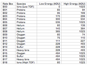 Table 11-1
Table 11-1: B boxes in normal mode In diagnostic mode, the boxes were:
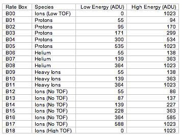 Table 11-2
Table 11-2: B boxes in diagnostic mode C Rates:
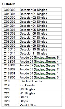 Table 11-3
Table 11-3: C Rates Notes: -"Singles" means single events on the named detector. HK Rates: These are various housekeeping values:
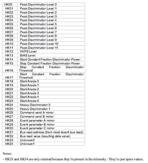 Table 11-4
Table 11-4: Housekeeping values Notes: - HK33 and HK34 are only retained because they're present in the telemetry. They're just spare values. J Rates: These are software counter totals: J00 Electron Events J01 Hi-E Ion Events J02 Low-E Ion Events J03 Electron Discards J04 Hi-E Ion Discards J05 Diagnostic Events J06 Diagnostic Discards L Rates:
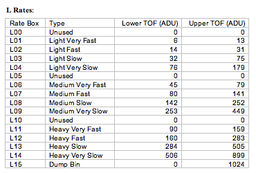 Table 11-5
Table 11-5: L Rates Notes: - Since the heavy ion discriminators appear to be of limited usefulness, the L Rate Boxes were reprogrammed after the Jupiter observing phase and are substantially different for the next observing phase of the mission. - Light events - neither heavy ion discriminator fired. - Medium events - H0 fired, H1 didn't - Heavy events - both discriminators fired. R Rates: R rates represent electron events. Rate Box Lower Energy (ADU) Upper Energy(ADU) R00 0,720 57,1023 R01 57 202 R02 203 719 Notes: - R00 nominally includes both low and high energies, but this is only a complication early in the Jupiter phase (days 6 - 22 of 2007), after which the electron detector threshold was raised so that only the high energies received valid events. This is why the L3 spectrograms put the electron pixels in the order: R01, R02, R00. - There are only 3 (out of 12) detectors dedicated to electrons (see figure 6). We number sectors the same way we do in the other rates, so electron rates only come from sectors: S00, S02, and S05. 11.4.3.5.1 Rate Box Definitions For Electrons and Low-Ions, the rate box definitions are simple ranges in Energy and TOF in ADUs which can be read found in the Level 2 headers. For Hi-Ions, the Rate Boxes are regions in the TOF-Energy plane (see figure 7). The precise specification of the rate boxes is complex and this is why we include rate box classifications in the Level 2 PHA data. However, for completeness, we include here the description of the Rate Box definition files. The binary files can be found in the instrument_config/ directory tree of the PEPSSI PDS data set. For each event packet that is not discarded, the 10-bit Energy ADU value is used as an index into a 1024-element array in which each element contains the 16-bit offset relative to the starting address of a "Rate Box" definition table. The offset is used in determining the beginning address of the corresponding row within the table. Each row contains a number of "break-points", and has the following format:
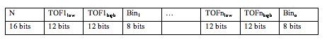 Table 11-6
Table 11-6: Row format N specifies the number of breakpoints contained in the row. The row whose address is contained in the energy pointer table entry identified by the event's Energy value is scanned to locate the first breakpoint whose TOFlow and TOFhigh values bracket the 11-bit TOF value from the event packet. The bin number contained in the 8-bit bin number field of the corresponding breakpoint identifies which one of 19 bins should be incremented in the histogram to which this event maps. A bin number of 0 corresponds to a background box. If the TOF value for the event does not fall within any of the breakpoints, then the event is treated as a background event and mapped to bin 0. 11.4.3.6 N2 and D_N2 N2 (and D_N2) are identical to their N1 counterparts except that they are typically sampled much more frequently (every 15 or 60 seconds) and only some of the L and C rates are present: - Only L01,02,03,04,08,09,13,14 are present - Only C00,02,03,05,06,07,08,09,10,13,14,15,16,17,22,23,24 are present 11.4.3.7 (D)_N(1/2)_STATUS All the STATUS extensions contain the same quantities for their respective coverage periods. STAT00 STATINT Status interval (seconds) STAT01 MACBLCKS Number of macro blocks fre STAT02 TLMVOL Telemetry volume produced STAT03 WTCHADDR Memory watch address STAT04 WTCHMEM Watched memory (pg. no) STAT05 WTCHDATA Watched memory STAT06 PEPSWVER Software version number STAT07 ALARMID Latest Alarm Id STAT08 ALARMTYP Latest alarm type STAT09 ALARMCNT Count of alarms STAT10 CMDEXEC Commands executed STAT11 CMDREJCT Commands rejected STAT12 MACEXEC Macro commands executed STAT13 MACREJCT Macro commands rejected STAT14 MACROID Id of most recent macro executed STAT15 MACROLRN Macro learn mode STAT16 MONRESP Monitor response STAT17 WRITEENB Memory write enable STAT18 HVPSCURR HVPS current STAT19 HVPSVOLT HVPS voltage STAT20 BIASCURR Bias current STAT21 BIASVOLT Bias voltage STAT22 PEPSTAT PEPSSI status word STAT23 DVOLTP5 +5V digital voltage STAT24 AVOLTN5 +5V analog voltage STAT25 VOLTP2 +2.5V voltage STAT26 VOLTN5 -5V voltage STAT27 VOLTP15 +15V voltage STAT28 VOLTN15 -15V voltage STAT29 DCURRP5 +5V digital current STAT30 ACURRP5 +5V analog current STAT31 CURRP2 +2.5 volt current STAT32 CURRN5 -5V current STAT33 CURRP15 +15V current STAT34 CURRN15 -15V current STAT35 PRIMCURR Primary current STAT36 LVPSTEMP LVPS temperature STAT37 ENGYTEMP Energy temperature STAT38 HVPSTEMP HVPS temperature STAT39 ADDR12C I2C read command address STAT40 RSLT12C I2C read command result 11.4.4 Bad Time Intervals (BTIs) Various instrument conditions can make the PEPSSI data difficult or impossible to use for scientific purposes. Powering down, ramping the high voltage power up or down, running in diagnostic mode, etc. will all make the PEPSSI data unusable for standard analysis. The "PEPSSI_BTI.txt" file contains a tab-separated list of "Bad Time Intervals" which should not be used for science analysis. It should be noted that the entire "Launch" phase of PEPSSI data is classified as a BTI. While not actually a BTI, the period between 2007 day 144 and day 178 should be treated with caution as well. The PEPSSI Rate Box tables were changed on day 144 and calibration and analysis of this period is still preliminary. 11.4.5 L3Data Format The L3 Files contain calibrated scientific data in an easily accessible form. There are three basic types of data in the L3 files: Quick-Look, flux-calibrated Rate Data, and calibrated PHA data. As with the L2 files, each file contains one UTC day's worth of data. No Diagnostic mode data is present in the L3 files. No "multi-hit" data is present in L3 files. Only N2-telemetered PHA data is present in L3 files. The Level 3 files are meant to be, as much as possible, self-documenting. All calibration constants, calibration formulas, and physical units should be present in the FITS header in an easily readable format. It should be possible, albeit with a lot of work, to reproduce the Level 3 files independently from the Level 2 files using the information in the Level 3 headers. 11.4.5.1 Primary HDU: Rate Weighted 2-D Histogram The image in the primary array of the L3 file is a rate-weighted 2-D histogram of the PHA data for that day binned in calibrated deposited energy. It represents a "best available" overview of the day's most detailed high energy ion data. The priority scheme distorts ion abundances, so we correct for that by using a "rate-weight" rather than a single count. For each period of 600 seconds, we divide the counts reported in the N2 rate box by the number of PHA events observed in that rate box. This is the weight those events are then assigned in constructing the histogram (see figure 8 for comparison of weighted and unweighted histograms). The two axes: energy deposited in the SSD and time of flight, are simple linear calibrations of the measured values. The calibration parameters are reported in the primary FITS header. 11.4.5.2 Quick Look Spectrograms The extensions: SPEC_Protons, SPEC_Helium, SPEC_Heavies, SPEC_Electrons, and SPEC_LowIon, contain quick-look spectrograms of their respective species. These spectrograms present counts/second N2 data, averaged over 60 second intervals and summed over all incidence directions (i.e. "Sectors"). 60 seconds is, except for the first hour of the day, the default accumulation interval of N2 data (Before 2007 day 42, the default N2 accumulation interval was 30 seconds). The x-axis of the spectrograms is hour of day. On the y-axis each pixel represents a different rate (e.g. B00, L01, R02, etc.). Nominal deposited energies of the rate boxes (or, in the case of Low-Ions, nominal time of flight bins) are given in the FITS header. 11.4.5.3 FLUX This HDU contains calibrated fluxes, uncertainties, and raw counts/sec rates for all of the High Energy Ion and Electron N2 Rate data. There is also an accumulation time column (DT) and three timing columns. IMPORTANT NOTE: The UTC YEAR and DAY_OF_YEAR columns are only included for convenience in plotting. DO NOT USE THEM for precise timing as there could be leap-second ambiguities in them. Use the ephemeris time (ET) column if precision is important. For some Rate Boxes, the exact particle species is undeterminable. They contain both Oxygen and Sulfur. Separate calibrations are supplied for Oxygen and for Sulfur. The Rate Box name is modified by appending an "O" or an "S" respectively in the FITS table column name. All of the quantities used in the calibration of the flux measurement, including their uncertainties are included in keywords in the FITS header. A description of the calibration procedure follows. IMPORTANT NOTE: Calibration work on the PEPSSI instrument is ongoing. Uncertainties in some quantities (particularly efficiency) are still very large. 11.4.5.3.1 FLUX Calibration Procedure We calculate the differential intensity j (1/cm2sr-s-keV) in terms of the counts C, time coverage T (s), geometric factor G (cm2sr), upper and lower energy bounds Ehi and Elo (keV), and detection efficiency eta, Equation 11-8.
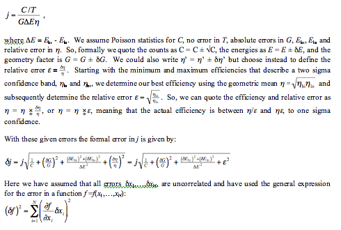 Equation 11-8
A "pseudo-code" version of the actual calculation code used is given in COMMENT keywords in the FITS header. Note on the correlation of the errors in E_lo and E_hi: To zeroth order, we can treat the errors on E_lo and E_hi as uncorrelated. One pragmatic reason is that it is a conservative assumption; if we are wrong then we are overstating the errors (at most by a factor of Root(2). Also, there are times when the uncertainty in E_lo or E_hi will be quite uncorrelated. For example the E_lo could depend on our understanding of the SSD threshold, while the E_hi could depend on our estimate of how fast the spectrum will be falling, both very different things. The most problematic case (from an error propagation point of view) would be where we believe we know the passband width delta(E) very well but we are not sure of the absolute energies. We think most of these potential cases are taken care of in the channel-to-Edeposit calibration (which establishes the scale) whereas most of the potential cases of uncorrelated errors in E_lo and E_hi occur in the E_deposit-to-E_incident calibration. 11.4.5.3.2 Derivation and Explanation of Calibration Table Values In this initial delivery of the PEPSSI data from the Launch and Jupiter phases of the New Horizons mission we have supplied values to convert the instrument specific data (e.g., count rates) into physical instrument-independent units (e.g., differential intensity), as well as computing the physical quantities themselves. It must be stressed that these are preliminary values that should not be used without significant effort from the user to understand the limitations (see section 11.4.5.3.1 for a description of the method used to calculate differential intensity, also called flux). The calibration quantities are energy pass-band (delta(E) = E_hi - E_lo, lower and upper limit of the energies of the particles measured), measurement efficiency (eta, the fraction of valid incident particles that are actually measured), the geometry factor (G, the measurement of the physical detector size and solid angle subtended by the field of view). These values are all given and applied with uncertainties in the Level 3 files. The energies are incident energies. Incident energy is the energy the particle has just before entering the instrument aperture absent the effect of the ~3 kV accelerating potential, which would induce a charge dependent energization. These energies were determined using a Monte Carlo technique that includes the energy loss as the particles trace through the entire system: start foil, free time-of-flight area, stop foil, dead layer, and energy defect. Losses through the foils are simulated and traced, as well as trajectory aberrations due to angular scattering. The energy defect for every particle and energy is also estimated by the SRIM code and checked with real data, where available. Some ground calibration of protons was also included. The uncertainties were not quantitatively determined from this modeling and measurements but are rather estimated from the known differences between various techniques. The geometry factors are derived from the same technique with similarly non-quantitative errors. These calibration values, although the uncertainties have not been estimated quantitatively, we consider appropriate to use for scientific study. The largest uncertainty in the calculated PEPSSI fluxes in the Level 3 data is due to the efficiency determination. PEPSSI, like most particle instruments (excluding sensors that rely only on solid state detectors and measure relative high ~> 1 MeV/nuc particles), is far from 100% efficient. This is due in large part to the "foil efficiency," which is the fraction of incident ions that result in secondary electrons that are detected by the micro channel plate (MCP). This efficiency is dependent on the voltage established across the MCP. So there are at least two primary physical processes involved (a) the probability that there are any secondary electrons emitted from the foil and (b) the probability that any resulting electrons are steered towards the MCP and multiplied to a sufficient current conducted to the anodes and that this signal triggers the start or stop disciminators. We can determine this through a combination of ground measurements, through analysis of the in-flight calibration alpha-particle source, modeling, and through intercalibration with known measurements. Before we can confidently report absolute fluxes, we must do all of these things. Currently we have only employed the final method, which has the obvious drawback of not providing an independent determination of the absolute flux. Therefore the fluxes provided in the Level 3 data should not be used as is to conduct science that is relying on absolute fluxes for scientific interpretation unless the user determines the fluxes independently and with full knowledge of the care that must be taken. In addition to these issues, a further consideration must be taken into consideration. The PEPSSI instrument was specifically engineered to make low rate measurements. This means that whenever there was a trade off between engineering effort, electronic components, power usage, mass, and volume, and ability to make high rate measurements, the later was given relatively low priority. For example, the CPU was selected for it's low power consumption, which means that there is an upper limit to the total number of events that can be processed. Therefore the user has to be aware that saturation of the rates can take place and that the saturation does not have to be uniform across different rates. It is possible during high rate periods for a large number of triple coincidence ions, for example, to impeded the processing of electrons. It is for this reason that it is very difficult to provide a single set of calibration values for this phase of the mission. We have provided what we have now and intend to continue to improve our knowledge and deliver the improved calibration information with subsequent updates to the PDS archive 11.4.5.4 PHA Data The three PHA extensions: PHA_ELECTRON, PHA_LOW_ION, and PHA_HIGH_ION contain the PHA event data. As in the L2 data, each row represents a single PHA event. Events with the multi-hit (cross talk) flag set have been excluded. Quantities of limited usefulness (such as Heavy Ion Discriminator triggers) have been excluded. Because of the difficulty of removing priority scheme biases from non-N2 PHA data, only N2 (APID == 0x692) PHA data is present in the L3 files. Calibrated Deposited Energy and/or Time of Flight values are given. The linear calibration constants and formulas are in the FITS headers. A Speed column is calculated from the Time of Flight assuming a 6.0cm flight path. The Rate Box classification for each event is given in the Rate_Box column. The PHA_HIGH_ION extension contains additional columns: The H_Incident_Energy, He_Incident_Energy, O_Incident_Energy, and S_Incident_Energy columns contain the calculated Incident energy assuming that the event is of that (H, He, O, or S) species. The Rate_Normalized_Weight column has removed Priority Group artifacts from the PHA data by the procedure described in the Primary HDU section above. This column is usually used in making histograms of the High Energy Ion PHA data. 11.4.6 Memory Required 1 GB memory and a 3 GHz Pentium is sufficient for processing. 11.4.7 Temporary File System Space Needed The Pre-Level 2 files require up to 50MB per day's worth of data. 11.4.8 Predicted Size of Output File(s) Level 2 files are in the range 1MB - 30MB. Level 3 files are typically 5-6 times larger than the corresponding Level 2 file, but only range up to a maximum of around 50MB. 11.4.9 Predicted Execution time Less than a minute per file, typically. The L1 to Pre-L2 conversion takes a few seconds per file. The entire Jupiter phase takes 40 minutes to convert from Pre-L2 to L2 and L3 files on a Red Hat Linux machine with 4 4GHz Xeon processors. It's not known how much parallelization was actually responsible for the speed. 11.4.10 Contact/Support Person(s) Stefano Livi, Matthew Hill, Martha Kusterer, Larry Brown and Reid Gurnee 11.4.11 Maintenance Schedule (Code/Data Updates, Documentation) As calibration data is collected during flight, the level 2 pipeline code will require updates either to calibration files or to code for bug fixes or enhancements.
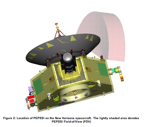 Figure 11-2: Location of PEPSSI on the New Horizons spacecraft. The
lightly shaded area denotes PEPSSI Field-of-View (FOV)
Figure 11-2: Location of PEPSSI on the New Horizons spacecraft. The
lightly shaded area denotes PEPSSI Field-of-View (FOV)
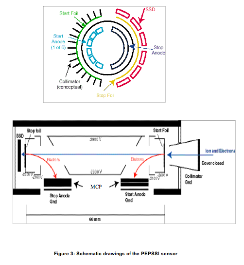 Figure 11-3: Schematic drawings of the PEPSSI sensor
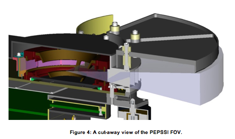 Figure 11-4: A cut-away view of the PEPSSI FOV.
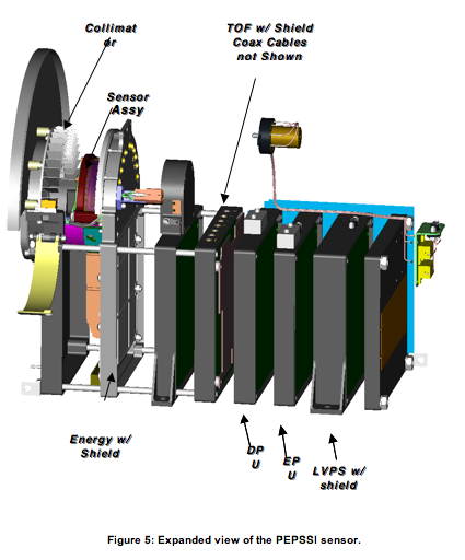 Figure 11-5: Expanded view of the PEPSSI sensor.
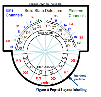 Figure 11-6: Pepssi Layout labelling
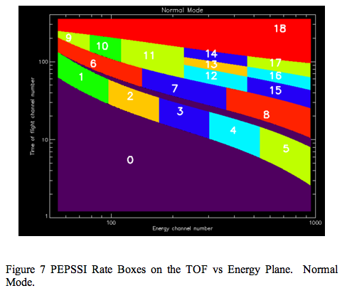 Figure 11-7: PEPSSI Rate Boxes on the TOF vs Energy Plane. Normal Mode.
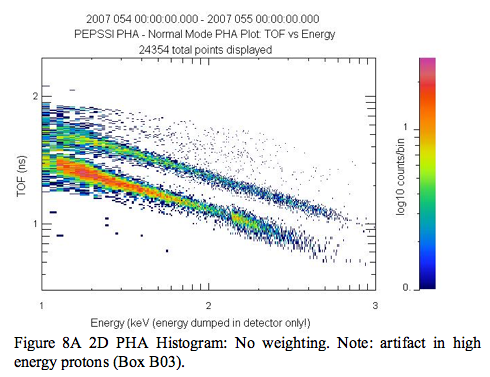 Figure 11-8A: 2D PHA Histogram: No weighting. Note: artifact in high
energy protons (Box B03).
Figure 11-8A: 2D PHA Histogram: No weighting. Note: artifact in high
energy protons (Box B03).
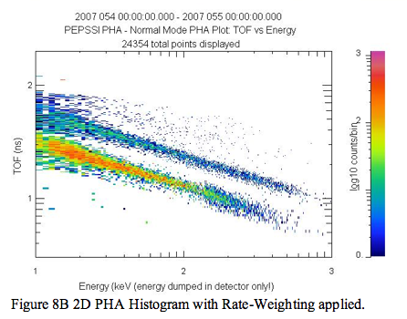 Figure 11-8B: 2D PHA Histogram with Rate-Weighting applied.
12. REX INSTRUMENT DESCRIPTION
12.1 Overview
The REX instrument is unique among the suite of instruments comprising
the New Horizons payload in that it is physically and functionally
incorporated within the spacecraft telecommunications subsystem.
REX consists of both a 'Flight Element' carried onboard the New
Horizons spacecraft, and a 'Ground Element' made up of existing
NASA Deep Space Network (DSN) transmitting and operations
facilities.
The primary purpose of the REX system is to investigate open questions
regarding the atmospheric and ionospheric structure, surface
conditions, and planetary radii of both Pluto and Charon. Secondarily,
New Horizons will attempt to observe any Kuiper Belt Objects (KBOs) it
encounters on its journey towards interstellar space . These
investigations fulfill many of the science objectives addressed in
NASA's Announcement of Opportunity (AO) document AO-OSS-01, which
defined the mission objectives for the Hew Horizons mission to Pluto.
REX is designed to fulfill the AO objectives by performing the
following distinct experiments:
1. A radio occultation experiment designed to detect and measure the
atmospheres and ionospheres of Pluto and Charon. The experiment
will be used to deduce, from phase changes in the uplink signal,
atmospheric temperature and pressure profiles down to the surface
of Pluto (and Charon, should it be found to have a tenable
atmosphere), and electron and ion densities of Pluto's (and
possibly Charon's) ionosphere.
2. A radiometry experiment, designed to measure the hemispherically
averaged surface emission brightness at a wavelength of 4.2 cm
(7.182 GHz, the nominal operating frequency of the New Horizons
radio). The dark-side emissions will be measured during the
occultation interlude. The day-side emissions will be measured as
is operationally feasible.
3. Accurate tracking of Doppler shifts in the transmission frequency
of the New Horizons transceiver will be used to deduce
gravitationally induced changes in velocity along the spacecraft's
flight path, thus measuring the gravitational fields of Pluto and
possibly Charon. The physics underlying these experimental
techniques and the details of the measurements themselves are
outlined in the New Horizons REX Users Manual.
The heart of the REX instrument is an Actel Field Programmable Gate
Array (FPGA) that takes samples of the downconverted & digitized
intermediate frequency (IF) receiver output and generates wideband
radiometer and narrowband sampled signal data products. The REX
hardware also includes an analog-to-digital converter (ADC) and other
direct interface components, and by extension all of the RF
telecommunications system hardware along the uplink (receive) path
from the High Gain Antenna (HGA) to the input to the ADC.
Stanford is responsible for the FPGA design and system analysis. APL
is responsible for the design of the telecommunications system and
incorporating the REX FPGA system therein.
The interfaces to the REX FPGA (see Fig. 12-1) include a 30 MHz clock
signal from the Ultra-Stable Oscillator, (USO), the secondary power
connections, the command and telemetry data interfaces to the Uplink
Card, the high-speed data interface to the Instrument Interface Card,
a 1 PPS signal for data framing, and the interface to the ADC, where
the wideband IF signal from the Uplink Card is sampled.
Figure 11-8B: 2D PHA Histogram with Rate-Weighting applied.
12. REX INSTRUMENT DESCRIPTION
12.1 Overview
The REX instrument is unique among the suite of instruments comprising
the New Horizons payload in that it is physically and functionally
incorporated within the spacecraft telecommunications subsystem.
REX consists of both a 'Flight Element' carried onboard the New
Horizons spacecraft, and a 'Ground Element' made up of existing
NASA Deep Space Network (DSN) transmitting and operations
facilities.
The primary purpose of the REX system is to investigate open questions
regarding the atmospheric and ionospheric structure, surface
conditions, and planetary radii of both Pluto and Charon. Secondarily,
New Horizons will attempt to observe any Kuiper Belt Objects (KBOs) it
encounters on its journey towards interstellar space . These
investigations fulfill many of the science objectives addressed in
NASA's Announcement of Opportunity (AO) document AO-OSS-01, which
defined the mission objectives for the Hew Horizons mission to Pluto.
REX is designed to fulfill the AO objectives by performing the
following distinct experiments:
1. A radio occultation experiment designed to detect and measure the
atmospheres and ionospheres of Pluto and Charon. The experiment
will be used to deduce, from phase changes in the uplink signal,
atmospheric temperature and pressure profiles down to the surface
of Pluto (and Charon, should it be found to have a tenable
atmosphere), and electron and ion densities of Pluto's (and
possibly Charon's) ionosphere.
2. A radiometry experiment, designed to measure the hemispherically
averaged surface emission brightness at a wavelength of 4.2 cm
(7.182 GHz, the nominal operating frequency of the New Horizons
radio). The dark-side emissions will be measured during the
occultation interlude. The day-side emissions will be measured as
is operationally feasible.
3. Accurate tracking of Doppler shifts in the transmission frequency
of the New Horizons transceiver will be used to deduce
gravitationally induced changes in velocity along the spacecraft's
flight path, thus measuring the gravitational fields of Pluto and
possibly Charon. The physics underlying these experimental
techniques and the details of the measurements themselves are
outlined in the New Horizons REX Users Manual.
The heart of the REX instrument is an Actel Field Programmable Gate
Array (FPGA) that takes samples of the downconverted & digitized
intermediate frequency (IF) receiver output and generates wideband
radiometer and narrowband sampled signal data products. The REX
hardware also includes an analog-to-digital converter (ADC) and other
direct interface components, and by extension all of the RF
telecommunications system hardware along the uplink (receive) path
from the High Gain Antenna (HGA) to the input to the ADC.
Stanford is responsible for the FPGA design and system analysis. APL
is responsible for the design of the telecommunications system and
incorporating the REX FPGA system therein.
The interfaces to the REX FPGA (see Fig. 12-1) include a 30 MHz clock
signal from the Ultra-Stable Oscillator, (USO), the secondary power
connections, the command and telemetry data interfaces to the Uplink
Card, the high-speed data interface to the Instrument Interface Card,
a 1 PPS signal for data framing, and the interface to the ADC, where
the wideband IF signal from the Uplink Card is sampled.
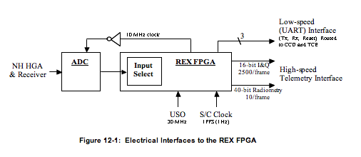 Figure 12-1: Electrical Interfaces to the REX FPGA
The input to the REX FPGA is normally the uplink signal from the DSN
after being filtered by a 4.5 MHz banpass filter (not shown) and
digitized by the ADC at a sample rate of 10 Msamples/s. The Input
Select function, commandable via uplink, allows the FPGA to process
any of seven predetermined digital signals for testing the FPGA
functionality (see the ROF Status Byte section below).
12.2 Raw Data Specifics
After receiving the command to start taking data, the REX FPGA, on the
1PPS strobe from the spacecraft clock, generates a continuous stream
of data containing In-Phase & Quadrature-Phase value pairs as well as
integrated radiometer values. This stream of data is divided into
fixed-length units called REX Output Frames (ROF) at a rate of one ROF
per 1.024 seconds. The ROFs are stored on the spacecraft solid state
recorder (SSR), and eventually played back via the High-Speed
Telemetry interface to the DSN and arrive at the SOC as raw telemetry
packets.
REX continues to produce ROFs until turned off. Each ROF contains
Time Tags that may be used to verify that a sequence of ROFs is a
contiguous set.
12.2.1 Raw Data Format
The SOC Raw pipeline decommutates each ROF from telemetry and places
it into the Primary Data Unit (PDU) of an individual FITS file. Each
PDU is stored as a one-dimensional image of 5088 bytes: the first
5082 bytes are the ROF; the last 6 bytes in the PDU are spare.
The SOC Raw pipeline also looks in the telemetry for packets
corresponding to the time of the ROF, and places them in EDU.
Specifically, data from spacecraft housekeeping ApIDs 0x004, 0x016,
0x084 and 0x096 as well as from Thruster packets are placed in EDUs 1
through 5, respectively, of the Raw FITS files.
12.2.1.1 PDU Content
Each ROF contains the items listed in Table 12-1 in an interleaved
format.
Figure 12-1: Electrical Interfaces to the REX FPGA
The input to the REX FPGA is normally the uplink signal from the DSN
after being filtered by a 4.5 MHz banpass filter (not shown) and
digitized by the ADC at a sample rate of 10 Msamples/s. The Input
Select function, commandable via uplink, allows the FPGA to process
any of seven predetermined digital signals for testing the FPGA
functionality (see the ROF Status Byte section below).
12.2 Raw Data Specifics
After receiving the command to start taking data, the REX FPGA, on the
1PPS strobe from the spacecraft clock, generates a continuous stream
of data containing In-Phase & Quadrature-Phase value pairs as well as
integrated radiometer values. This stream of data is divided into
fixed-length units called REX Output Frames (ROF) at a rate of one ROF
per 1.024 seconds. The ROFs are stored on the spacecraft solid state
recorder (SSR), and eventually played back via the High-Speed
Telemetry interface to the DSN and arrive at the SOC as raw telemetry
packets.
REX continues to produce ROFs until turned off. Each ROF contains
Time Tags that may be used to verify that a sequence of ROFs is a
contiguous set.
12.2.1 Raw Data Format
The SOC Raw pipeline decommutates each ROF from telemetry and places
it into the Primary Data Unit (PDU) of an individual FITS file. Each
PDU is stored as a one-dimensional image of 5088 bytes: the first
5082 bytes are the ROF; the last 6 bytes in the PDU are spare.
The SOC Raw pipeline also looks in the telemetry for packets
corresponding to the time of the ROF, and places them in EDU.
Specifically, data from spacecraft housekeeping ApIDs 0x004, 0x016,
0x084 and 0x096 as well as from Thruster packets are placed in EDUs 1
through 5, respectively, of the Raw FITS files.
12.2.1.1 PDU Content
Each ROF contains the items listed in Table 12-1 in an interleaved
format.
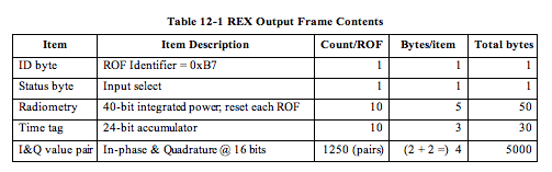 Table 12-1
Table 12-1: REX Output Frame Contents 12.2.1.1.1 ROF ID byte The ID byte is the first byte in the ROF and should always have the same value; see Table 12-2.
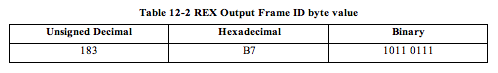 Table 12-2
Table 12-2: REX Output Frame ID byte value 12.2.1.1.2 ROF Status byte The ROF Status byte is the fourth byte in the ROF. In bit positions 6, 5 & 4 it contains the three bits that make up the Input Select setting for the ROF; all other bits are normally zero. When Input Select is set to any of its non-zero values, the ADC output is replaced as the FPGA input with a predetermined 10Msample/s signal as described in Table 12-3. In that case, the ouptut of the REX FPGA should be deterministic and known, and may be compared bit-for-bit against the expected ouput as a limited check on the health of the FPGA as well at that of the Input Select system.
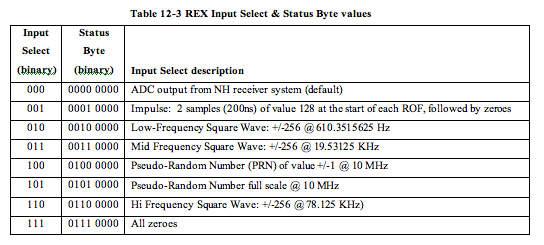 Table 12-3
Table 12-3: REX Input Select & Status Byte values 12.2.1.1.3 Integrated Radiometry values The details of how incoming power is used as radiometry are given in Tyler et al., 2007. The FPGA integrates the incoming power from its input signal by squaring and summing the ~10Msamples/s that compose its input. Ten accumulating radiometry values are stored in each ROF, and the FPGA resets the value to zero at the start of each ROF. Each radiometry value comprises 40 bits, or 5 bytes, as an unsigned integer, and the bytes are in MSByte-first order, interleaved with I&Q values. The time interval between radiometry values is one-tenth of a ROF or 102.4ms. In each ROF, REX stores a integrated radiometry value at the start time of that ROF (and not 102.4ms after its start), so the tenth, or last, radiometry value of associated with a ROF (i.e. the one that represents a full 1.024s of integration time) is actually stored as the first radiometry value in the following ROF. 12.2.1.1.4 Time Tag values REX places ten incrementing time tags in each ROF. The first time tag of the first ROF after a start command is zero, and the following time tags increment by one. Unlike the integrated radiometry values, the time tag is not reset at the start of each ROF. Each time tag values comprises 24 bits, or 3 bytes, as an unsigned integer, and the bytes are in MSByte-first order, interleaved with I&Q values. Each increment of the time tag represents 102.4ms, so the rollover time is just under a fortnight and a half. The time tags can be used both to identify any breaks in a sequence of ROFs, and to determine the time between any two ROFs in a sequence. 12.2.1.1.5 I & Q value pairs Each ROF contains 1250 pairs of In-Phase (I) & Quadrature-Phase (Q) values. Each I value and each Q value comprises 16 bits or two bytes as a twos-complement signed value. The process of down conversion from 10 Ms/s is accomplished by heterodyning to zero frequency the uplink carrier signal centered initially at the 2.5MHz Intermediate Frequency (IF) center frequency, followed by use of time-invarient baseband filters to reduce the bandwidth. The details are too extensive to include here, but are explained in detail in Tyler et al. (2007). 12.2.1.2 PDU Data layout: Interleaving In each ROF, the bytes of the ID, Status, Radiometry and Time Tag values are interleaved with the I&Q value pairs, but none of the values start or end on other than a byte boundary. There are two ways to describe such an arrangement: describe the layout of the ROF as built out of a sequence of bytes extracted from the de-interleaved data values (ID, Status, Radiometry, Time Tag, I&Q); describe the layout of the data values as a sequence bytes from the ROF. Both methods will be used here, the latter first as it lends itself more easily to writing computer code to extract the data values from the ROF. Indeed, an IDL(tm) routine to extract ROF data value exists with less than two dozen lines. The I&Q value pairs use up over 98% of the space in each ROF; this suggests that describing the data layout of the other data values will take less time and leave the I&Q values as "everything else."
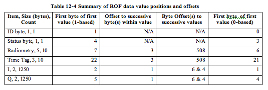 Table 12-4
Table 12-4: Summary of ROF data value positions and offsets This section uses the notation in Table 12-5 to describe and or locate the various quantities in the ROF:
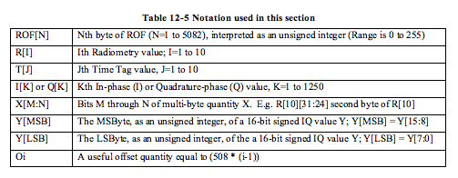 Table 12-5
Table 12-5: Notation used in this section 12.2.1.2.1 Layout of ID & Status bytes The ID and Status bytes are the first and fourth bytes in the ROF, respectively, and can simply be obtained from the ROF as such as there are no following bytes or values: ID byte = ROF[1] Status byte =ROF[4] 12.2.1.2.2 Layout of Radiometry The first byte of the first radiometry value is the seventh byte of the ROF, and the following four bytes of that first radiometry value are each offset by three bytes from the previous byte. The order is MSByte-first. So, the first radiometry value of a ROF may be calculated from the following formula: R[1] = ( ( (ROF[7] * 256 + ROF[10]) * 256 + ROF[13]) * 256 + ROF[16]) * 256 + ROF[19] The following radiometry values' bytes in the same ROF are each offset 508 bytes from the previous radiometry value's bytes. So, more generally: R[i]=(((ROF[7+Oi]*256 + ROF[10+Oi])*256 + ROF[13+Oi])*256 + ROF[16+Oi])*256 + ROF[19+Oi] 12.2.1.2.3 Layout of Time Tags The first byte of the first time tag value is the 22nd byte of the ROF, and the following two bytes of that first radiometry value are each offset by three bytes from the previous byte. The order is MSByte-first. So, the first time tage value of a ROF may be calculated from the following formula: T[1] = (ROF[22] * 256 + ROF[25]) * 256 + ROF[28] The following time tag values' bytes in the same ROF are each offset 508 bytes from the previous radiometry value's bytes. So, more generally: T[i] = ( ROF[22+Oi] * 256 + ROF[25+Oi] ) * 256 + ROF[28+Oi] 12.2.1.2.4 Layout of I & Q values The bytes that are used to store the I & Q values alternate in sequence (I[1], Q[1], I[2], Q[2], I[3], Q[3], ..., I[1250], Q[1250]) as 16-bit MSByte-first two's complement signed integers, that cover all of the bytes not used by the other values (ID, Status, Radiometry, Time Tags) above. Specifically, Table 12-6 describes how ROF bytes are used to calculate I[K] and Q[K] for K=1 to 1250:
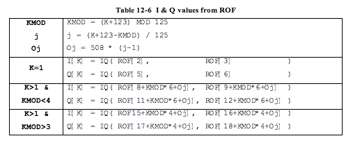 Table 12-6
Table 12-6: I & Q values from ROF Where Function IQ(MSByte,LSByte) is defined as (with MSByte & LSByte interpreted as unsigned 8-bit - i.e. 1-byte - integers) IQ(MSByte,LSByte) = 256 * MSByte + LSByte if MSByte is between 0 and 127 inclusive. Otherwise, it is defined as IQ(MSByte,LSByte) = 256 * MSByte + LSByte - 65536 12.2.1.3 Layout of ROF The tables below have one cell per ROF byte, and indicate which data values (ID, Status, Radiometry, &c) each byte contributes to. The order of bytes in these table is left-to-right and down i.e. ROF[1] ROF[2] ROF[3] ROF[7] ROF[8] ROF[9] ROF[10] ... ... The first six ROF bytes contain the ID & Status bytes and the first I&Q pair: ID I[1][MSB] I[1][LSB] Status Q[1][MSB] Q[1][LSB] The next 508-byte "chunk" (ROF byte order is left-to-right then down) contains one Radiometry value, one Time Tag, and 125 I&Q pairs: R[1][39:32] I[2][MSB] I[2][LSB] R[1][31:24] Q[2][MSB] Q[2][LSB] R[1][23:16] I[3][MSB] I[3][LSB] R[1][15:8] Q[3][MSB] Q[3][LSB] R[1][7:0] I[4][MSB] I[4][LSB] T[1][23:16] Q[4][MSB] Q[4][LSB] T[1][15:8] I[5][MSB] I[5][LSB] T[1][7:0] Q[5][MSB] Q[5][LSB] I[6][MSB] I[6][LSB] Q[6][MSB] Q[6][LSB] I[7][MSB] I[7][LSB] Q[7][MSB] Q[7][LSB] I[8][MSB] I[8][LSB] Q[8][MSB] Q[8][LSB] ... ... I[126][MSB] I[126][LSB] Q[126][MSB] Q[126][LSB] The rest of the ROF comprises 9 more chunks of 508 bytes per chunk, essentially identical to the one above, incrementing the R[] & T[] indices by one per chunk, and incrementing the I[] & Q[] indices by 125 per chunk. Each chunk except the last contains 125 I&Q pairs; N.B. the tenth chunk ends after its 504th byte and after its 124 I&Q pair which is the 1250th, and last, I&Q pair of the ROF. 12.2.2 Data Sources (High/Low Speed, CCSDS, ITF) REX data are in the high-speed stream and come to the SOC in CCSDS packets. 12.2.3 Definition of an "Observation" One REX Output Frame (ROF), as defined above, is an observation. 12.2.4 Housekeeping in Raw FIT files' extensions The Raw pipeline puts information from several types of housekeeping (HK) packets into Extension Data Units (EDUs) 1 through 5 (see Table 12-7). The pipeline attempts to find the closest HK packet to the observation time. If no packet is available, the EDU is not present and the corresponding Extension Header Unit (EHDU) will indicate a zero-sized EDU.
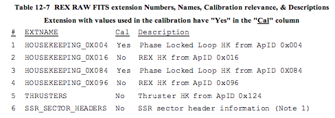 Table 12-7
Table 12-7: REX RAW FITS extension Numbers, Names, Calibration relevance, & Descriptions Extension with values used in the calibration have "Yes" in the "Cal" column. Note 1: The SSR Sector Header information is only present in REX data with ApID 0x7b1 in the FITS filename. The presence of ApID 0x004 housekeeping indicates Side A is active, and the presence of ApID 0x084 housekeeping indicates Side B is active. If neither 0x004 nor 0x084 housekeeping is present, then the data will not be calibrated. 12.2.5 Raw Science Data and/or Housekeeping Requirements Radio receiver housekeeping (ApIDs 0x004 and/or 0x084 noted above). 12.3 Calibration Specifics 12.3.1 Calibration Algorithms The conversion of RAW REX data to Calibrated data is concerned with two data streams from REX: (1) the REX filter output, comprising 16-bit samples at 1250 samples (complex) per ROF, i.e., 1250 In-phase samples per ROF and 1250 Quadrature-phase samples per ROF, and (2) the Radiometer output, comprising 40-bit samples at a rate of 10 samples per ROF, and (3) the Time Tag 12.3.1.1 Calibrating the REX filter output: In-phase & Quadrature-phase values The conversion of the I/Q samples from the raw DN to calibrated physical units (milliVolts) involves applying a gain independent scaling, since the FIR process producing the samples has no adjustable parameters. The algorithm takes each two ROF bytes that represent a single filter output value and does the following: 12.3.1.1.1 Combine the unsigned bytes into a two's complement 16-bit signed integer filter value FilterValue = ( I[MSB] * 256 ) + I[LSB] IF FilterValue > 32767 THEN FilterValue = FilterValue - 65536 The example above is for In-Phase filter values; the procedure for Quadrature-phase values is identical. 12.3.1.1.2 Scale the filter value by the calibrated reference voltage VIorQ = (1000 / (2^15)) * FilterValue N.B. As noted below, this scaling factor is only stored in the FITS EHDU for these data, and the 16-bit data values are what are stored in the EDU calibrated FITS file. 12.3.1.2 Calibrating the REX Radiometry The formula for converting the Raw REX radiometer data to power, in units of dBm, is as follows: Prad = -172 + 10 * log10(sample) - Ro - (AGC - AGCoffset) * dBstep Where sample = Combined unsigned integer value of five radiometry bytes from ROF AGC = AGC Voltage from whichever REX Side, A or B, is active - REX side A active => CDH_PLL_AGCV_1 from ApID 0x004 - REX side B active => CDH_PLL_AGCV_2 from ApID 0x084 - The calbration pipeline uses whichever ApID is in the Raw FITS file extensions AGCoffset = REX Side-dependent constant AGC Voltage offset: 2512 if Side A; 2504 if Side B. Ro = Constant: 96.870 dBstep = Constant: 0.475 Since the Radiometry is integrating, or accumulating, instantaneous power values and saving ten accumulations per ROF, only the tenth value, integrated over the full ROF of about 1s, can be thought of as being in units of dBm or dB relative to 1mW. All of the previous values should be divided by the time since the accumulation was reset. Also, it was noted above that the tenth accumulated value for each ROF is actually stored as the first Radiometry value in the next ROF. Perhaps units of dBj would be more accurate. The formula for dBm above can be rearranged to convert the Raw value to mW as follows: Prad_mW = sample * 10-(172 + Ro + (AGC - AGCoffset) * dBstep) / 10 OR Prad_mW = sample * K where K = 10-(172 + Ro + (AGC - AGCoffset) * dBstep) / 10 and all other symbols are the same as above. N.B. As noted below, the scaling factor K is only stored in the FITS header for these data, and the 40-bit data values for sample, in double precision IEEE form, are what are physically stored in the calibrated FITS file. 12.3.1.3 Calibrating the REX Time Tags The time tags are 24-bit integers that increment ten times per ROF frame of 1.024s and represent the time since the first contiguous ROF frame in a sequence (or, in the unlikely case of REX taking data for more than about a fortnight and a half, from the last Time Tag rollover), so the formula to convert from the 24-bit Time Tag value TTraw to seconds is Ts = TTraw * 0.1024 N.B. As noted below, the scaling factor 0.1024 is only stored in the FITS header for these data, and the 24-bit data values for TTraw, in double precision form, are what are stored in the calibrated FITS file. 12.3.2 Calibrated FITS file data format The calibrated data from each ROF are stored in a single FITS file. The PDU is empty, and all data are stored in FIT extensions. This section gives the details of the extensions. 12.3.2.1 Extension Data Unit (EDU) 1: I & Q values The first extension of the Calibrated FITS file is a FITS BINTABLE, or binary table, containing the calibrated I&Q value pairs in mV. The table has two columns (I & Q) and 1250 rows. N.B. Because the conversion from the raw integer form to the calibration unit of mV is a linear factor, the values physically stored in the Calibrated FITS file are the 16-bit integer results of the first step of the calibration described above. The scaling factor applied in the calibration is actually only stored in the FITS BINTABLE header TSCALn keywords. From there, most FITS readers will apply the factor when reading the data, but any user writing their own FITS reading software should be aware of the presence and application of this scaling factor. 12.3.2.2 EDU 2: Radiometry & Time Tags The second extension of the Calibrated FITS file is also a FITS BINTABLE, containing the ROF's Radiometry values in dBm, the Time Tags in seconds, and the Radiometry values in mW. The table has thre columns (Radiometry in dBm; Time Tags in seconds, and Radiometry in mW). N.B. Because the conversion from the raw integer form to the calibration unit of seconds and mW in the second and third columns (but not dBm) is a linear factor, the values physically stored in the Calibrated FITS file are the integral values from combining the Raw bytes, stored as double precision IEEE floating point numbers. The scaling factors applied in the calibration is actually only stored in the FITS BINTABLE header TSCALn keywords. From there, most FITS readers will apply the factor when reading the data, but any user writing their own FITS reading software should be aware of the presence and application of this scaling factor. 12.3.2.3 Additional FITS Extensions (planes) and Their Definitions After EDUs 1 & 2, any extensions (housekeeping, thrusters, SSR info), from the Raw FITS file for each ROF are carried over to the corresponding Calibrated FITS file. Table 12-8 describes those extensions.
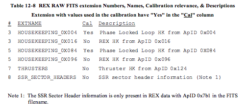 Table 12-8
Table 12-8: REX RAW FITS extension Numbers, Names, Calibration relevance, & Descriptions 12.3.2.4 Scientific Units The units of the calibrated values, after applying the scaling factors if present, are as follows: Filter output: Voltage (mv) Radiometry: Power (dBm and mW) Time Tag: Time (s) 12.3.2.5 Additional FITS and PDS Keywords 12.3.2.5.1 Radiometry calibration provenance added to PHDU A summary of the Radiometry calibration is added to the Primary Header Data Unit (PHDU), using the prefix RAD for the keywords. The information in this summary includes - the formula - the AGC voltage - which REX side was assumed to be active (A or B) - the value of all constants used in the formula (AGCoffset, Ro, dBstep). 12.3.2.5.2 FITS keywords added to EHDU 1 The average power, the ID byte, the Status byte and a decoded version of the Status byte (indicating the input select setting) are added to EHDU 1. 12.3.2.5.3 Scaling parameters As noted above, the linear calibrations are achieved by physically placing the Raw integer values into the FITS binary tables and providing scaling factors (FITS keyword TSCALn) in the corresponding EHDUs. These scaling parameters are also present in the PDS labels for the PDS archive (PDS keyword SCALING_FACTOR). 12.3.3 Hardware/OS Development Platform PC/Linux 12.3.4 Language(s) Used IDL 12.3.5 Third Party Libraries Required cfitsio (if C used) or ASTRO (if IDL used) 12.3.6 Calibration Files Needed (with Quantities) None; all calibration factors are in the source code and listed above. 12.3.7 Memory Required < 128MB 12.3.8 Temporary File System Space Needed None. 12.3.9 Predicted Size of Output File(s) < 70 Kbyte 12.3.10 Predicted Execution time Less than a second per ROF 12.3.11 Contact/Support Person(s) Ivan Linscott 12.3.12 Maintenance Schedule (Code/Data Updates, Documentation) None planned; something may come out of the PDS review. 13. SDC INSTRUMENT DESCRIPTION 13.1 Overview The mission of the Venetia Burney Student Dust Counter (VSDC) is to analyze the size and distribution of dust particles along the New Horizon's trajectory to the Kuiper Belt. The SDC instrument consists of the front end analog electronics, the digital interface electronics, the detector panel, and the intraharness. Each particle impact on one of the 12 active SDC detectors will be a candidate for a science event. This impact causes a depolarization signal in the Polyvinylidene Flouride (PVDF) detector film dependent on the size and speed of the particle. This signal gets converted to a digital number via the electronics. If the amplitude is above the value at which the threshold is currently set, then the signal is stored in memory as a science event along with other relevant housekeeping data. These depolarization signals are measured in charge (Q) produced (Note that SDC reports charge in number of electrons. Even though this is not strictly charge, the number of electrons will from here on be re- ferred to as the charge). The charge from an impacting particle depends on the particles mass and velocity. Because the unit of the raw data is data number (DN), a calibration curve from data number to charge (DN=>Q) is needed. This curve is a function of box temperature and detector channel. For SDC, this curve was produced pre-flight and is checked during the mission with internal calibration procedures. The DN=>Q calibration curves are shown in Figure 13-7. The calibrated files are derived from the raw files through these curves. 13.2 Raw Data Specifics The raw data are unprocessed telemetry. At the SOC and PDS, all levels of data are recorded in FITS format. The SDC team uses IDL for our data processing and hence would like to be able to load these FITS files into IDL as structures/arrays, etc. To do this we typically use an IDL fits reader which can be found in the Goddard IDL library. Specifically we use mrdfits.pro. If this is used, please note that a "/unsigned" flag must be given as the data are all unsigned integers. The raw data FITS file consists of housekeeping and science data. Some of these data are not used in the calibration process to produce the calibrated data. It stated in the PDS label files which telemetry points are and are not used by the calibration process. In addition to the IDL functions for FITS files, generic programs such as fv can also be found. If opened in this program, the raw data tables are displayed as in figure below.
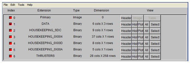 Figure 13-1: Raw data tables as viewed by Fv.
13.2.1 Data Format
The data in the FITS file are stored as a binary table extension.
There are five tables in the raw file. These tables and their
columns are :
DATA -
1) Copy Number - Not used in calibration
2) Channel ID - Detector number (0-13) [Channel 10 has a
electrical issue and is not used for science. Channels 6 and 13 are
reference detectors. These detectors cannot detect real dust as they
are covered. For all higher level data products the channel IDs are
incremented by one and become 1-14.]
3) Zero Fill - Not used in calibration
4) Threshold - First note that this DN scale is reversed. This
means 65535 is a small event while 0 is a very large event. This
reverse scale is also true for the Magnitude described below. The
threshold value is the maximum (highest DN but smallest signal)
magnitude (see next item) for accepted hits. Hits above (smaller
amplitude) the threshold are rejected at the instrument level. These
thresholds are adjustable and vary from channel to channel. [Note
that it is SOMETIMES possible for a slightly smaller amplitude hit to
come in just above this value due to the way the software works].
5) Magnitude - The size of the hit in DN [Note that this scale is
also reversed. This means that 65535 is a small event while
0 is a very large event.]
6) Time Stamp - The time the hit was recorded in Mission Elapsed
Time (MET)
HOUSEKEEPING_SDC -
1) MET - Mission Elapsed Time
2) PanTemp A-D - Temperature recorded on the panel of SDC
3) BoxTemp 1-4 - Temperatures recorded on the electronics box of SDC
HOUSEKEEPING_0X004 - Values used in Calibration from this table:
1) CDH_PNL_A-D_TEMP - Temperature recorded on the panel of SDC
(Note these are the same as above)
2) CDH_ANA_A-B_TEMP - Temperature recorded on analog side of the
electronics box of SDC
3) CDH_ANA_DCDC_TEMP - Temperature recorded on DCDC
4) CDH_ANA_DCDC_TEMP - Temperature recorded on the FPGA
HOUSEKEEPING_0X00D - Values used in Calibration from this table:
d. MET - Mission Elapsed Time for the columns in this table
e. CDH_TEMP_SDC_ELEC - Electronics box temperature as recorded by
the spacecraft
f. CDH_TEMP_SDC_DET - Detector temperature as recorded by the spacecraft
HOUSEKEEPING_0X00A
1) MET - Mission Elapsed Time for the columns in this table
2) SDC_LVPS_VOLT - Voltage of SDC recorded by the spacecraft
3) SDC_LVPS_CURR - Current of SDC recorded by the spacecraft
THRUSTERS - Values used in this Table
- GC1_DATA_VALID_MET - MET of Thruster Fire
- GC1_RCS_FIRE_MINOR_1-24 - Tells whether one of the thrusters fired
13.2.2 Data Sources (High/Low Speed, CCSDS, ITF)
SDC data are low-speed CCSDS packets only.
13.2.3 Definition of an "Observation"
One observation is one collection of events in one CCSDS packet.
13.2.4 Housekeeping Needed in Level 1 Files (for Calibration)
See Section 13.2.1
13.2.5 Raw Science Data and/or Housekeeping Requirements
From launch to the end of the first month, HK packet METs should be
within 1 minute of a dust observation
From the end of the first month until Jupiter, HK packet METs should
be within 1 hour
From Jupiter until the end of the mission HK packet METs should be
within 1 day
For the redundant points, such as temperatures, only one of these
needs to satisfy this requirement.
13.2.6 Notes about Raw Data
1) The scale in DN is "backwards" on a 0-65535 scale. In other
words, a very large hit represent a number near 0. A small hit
registers as a number close to 65535
2) The threshold can be tuned and represents the minimum DN of a
detectable hit. HOWEVER, it is possible due to the way the
electronics work, that you might get a hit with a slightly
higher DN (smaller hit) than the threshold. Usually this is
no more than a few tens of DN higher than the threshold.
3) SDC has on-board flight rules for autonomously turning a
channel off. The user will then need to know when the
channel was on/off. This information is in a separate file
named sdc_on_off_times.dat.
4) The maximum number of recorded hits in one second on a given
channel for SDC is in general 3. The way the timing works
it is possible to get up to 5 hits/second. However, if more
than one hit is recorded in one second (instrument wide)
this is considered a coincident event and will be flagged.
The science processing interprets such an event as s/c noise
and removes it.
13.3 Calibration
The data calibration is a three-step process. The telemetry is stored
as raw DN. Each DN value representing the size of a hit is converted
into charge (see below). Mass is then derived from this charge via
the ground calibration results obtained at a dust accelerating
facility.
13.3.1 Pre-Flight Calibration Procedure- Charge
In a temperature controlled environment, the electronics from the end
of the PVDF to the DN in the raw data were calibrated, at each of 4
calibration box temperatures and for each of the 14 channels. This
was done by injecting 19 (actually 21; see below) fixed-amplitude
charge pulses 100 times into a channel and recording the DN value each
time. From those recorded values, the average DN (DNavg) and its
standard deviation (SIG) at each charge pulse amplitude, box
temperature and channel were calculated. Then, for each box
temperature and channel, a 9th order polynomial fit of Q(DNavg) was
derived. Finally, these 3 sets of values (the polynomial
coefficients, DNavg, and SIG) were stored in a matrix. This matrix
contains all information required to calculate the charge equivalent
to a DN as a function of box temperature and channel (detector), as
well as the uncertainty in that calculated charge value.
For detailed information about this calibration procedure see Horanyi,
et. al., "The Student Dust Counter on the New Horizons Mission", Space
Sci. Rev., in pub., 2007..
--Charge Calibration File--
The calibration file contains the calibration values described above
as a matrix of floating point values with dimension (4 X 14 X 3 X 19)
representing values for the 4 box temperatures (Tbox), the 14
channels, and the 3 types of calibration values (coefficients, DN_avg &
SIG). The the zero-based indices have the following meanings:
First Index - 4 Box Temperatures:
0) 49.9deg
1) 40deg
2) 34.25deg
3) -7.1deg
Second Index - 14 Channels
0) First channel
1) Second channel
...
13) Last (fourteenth) channel
Third Index - 3 types of data.
- By setting this index you select which array of values are retrieved
via the last index:
0 - Coeffs - Polynomial fit coefficients (in practice only the
first 10 are used)
1 - DNavg - Average DN recorded during Calibration at this Tbox & Channel
2 - SIG - Standard deviation of the corresponding average DN value
(index = 1)
Fourth Index - Dependent on Third index; see also Note 1 below
- For the coefficients of the polynomial (third index = 0)
log10(Q(DN)) = C0 + C1*DN + C2*DN2 + C3*DN3 + ... + C9*DN9
- 0) Zeroth order coefficient, C0
- 1) First-order coefficient, C1
- N) Nth-order coefficient, Cn
- For DN_avg & SIG data types (third index = 1 & 2)
- the index of each charge pulse tests arranged in order of
increasing charge (decreasing DN)
Note 1: We injected charge pulses at 21 different values, but some of
these were too small to record, and no channel had more than 19
recordable values at any box temperature. Also, there are only 10
coefficients in the 9th-order polynomial. So, although the matrix can
hold up to 19 coefficients, average DNs or standard deviations per box
temperature and channel, only the derived/recorded values are stored
in the matrix, and the any unused matrix values are set to zero. This
does not affect the polynomial evaluation, but when using the DNavg
and SIG values one should ignore zero values.
Thus from this matrix you can get 3 things: Fit coefficients, Average
DNs, and standard deviations.
So, for example, to get the fit coefficients for a box temperature of
-7.1 degrees on the first channel you want (-7.1, first channel,
Coeff, *) => CALARRAY[3, 0, 0, *] (IDL notation). See Figure 13-7 for
a plot of Charge vs DN represented by the Fit Coefficients.
For detailed information about this calibration procedure see Horanyi,
et. al., "The Student Dust Counter on the New Horizons Mission", Space
Sci. Rev., in pub., 2007.
Figure 13-1: Raw data tables as viewed by Fv.
13.2.1 Data Format
The data in the FITS file are stored as a binary table extension.
There are five tables in the raw file. These tables and their
columns are :
DATA -
1) Copy Number - Not used in calibration
2) Channel ID - Detector number (0-13) [Channel 10 has a
electrical issue and is not used for science. Channels 6 and 13 are
reference detectors. These detectors cannot detect real dust as they
are covered. For all higher level data products the channel IDs are
incremented by one and become 1-14.]
3) Zero Fill - Not used in calibration
4) Threshold - First note that this DN scale is reversed. This
means 65535 is a small event while 0 is a very large event. This
reverse scale is also true for the Magnitude described below. The
threshold value is the maximum (highest DN but smallest signal)
magnitude (see next item) for accepted hits. Hits above (smaller
amplitude) the threshold are rejected at the instrument level. These
thresholds are adjustable and vary from channel to channel. [Note
that it is SOMETIMES possible for a slightly smaller amplitude hit to
come in just above this value due to the way the software works].
5) Magnitude - The size of the hit in DN [Note that this scale is
also reversed. This means that 65535 is a small event while
0 is a very large event.]
6) Time Stamp - The time the hit was recorded in Mission Elapsed
Time (MET)
HOUSEKEEPING_SDC -
1) MET - Mission Elapsed Time
2) PanTemp A-D - Temperature recorded on the panel of SDC
3) BoxTemp 1-4 - Temperatures recorded on the electronics box of SDC
HOUSEKEEPING_0X004 - Values used in Calibration from this table:
1) CDH_PNL_A-D_TEMP - Temperature recorded on the panel of SDC
(Note these are the same as above)
2) CDH_ANA_A-B_TEMP - Temperature recorded on analog side of the
electronics box of SDC
3) CDH_ANA_DCDC_TEMP - Temperature recorded on DCDC
4) CDH_ANA_DCDC_TEMP - Temperature recorded on the FPGA
HOUSEKEEPING_0X00D - Values used in Calibration from this table:
d. MET - Mission Elapsed Time for the columns in this table
e. CDH_TEMP_SDC_ELEC - Electronics box temperature as recorded by
the spacecraft
f. CDH_TEMP_SDC_DET - Detector temperature as recorded by the spacecraft
HOUSEKEEPING_0X00A
1) MET - Mission Elapsed Time for the columns in this table
2) SDC_LVPS_VOLT - Voltage of SDC recorded by the spacecraft
3) SDC_LVPS_CURR - Current of SDC recorded by the spacecraft
THRUSTERS - Values used in this Table
- GC1_DATA_VALID_MET - MET of Thruster Fire
- GC1_RCS_FIRE_MINOR_1-24 - Tells whether one of the thrusters fired
13.2.2 Data Sources (High/Low Speed, CCSDS, ITF)
SDC data are low-speed CCSDS packets only.
13.2.3 Definition of an "Observation"
One observation is one collection of events in one CCSDS packet.
13.2.4 Housekeeping Needed in Level 1 Files (for Calibration)
See Section 13.2.1
13.2.5 Raw Science Data and/or Housekeeping Requirements
From launch to the end of the first month, HK packet METs should be
within 1 minute of a dust observation
From the end of the first month until Jupiter, HK packet METs should
be within 1 hour
From Jupiter until the end of the mission HK packet METs should be
within 1 day
For the redundant points, such as temperatures, only one of these
needs to satisfy this requirement.
13.2.6 Notes about Raw Data
1) The scale in DN is "backwards" on a 0-65535 scale. In other
words, a very large hit represent a number near 0. A small hit
registers as a number close to 65535
2) The threshold can be tuned and represents the minimum DN of a
detectable hit. HOWEVER, it is possible due to the way the
electronics work, that you might get a hit with a slightly
higher DN (smaller hit) than the threshold. Usually this is
no more than a few tens of DN higher than the threshold.
3) SDC has on-board flight rules for autonomously turning a
channel off. The user will then need to know when the
channel was on/off. This information is in a separate file
named sdc_on_off_times.dat.
4) The maximum number of recorded hits in one second on a given
channel for SDC is in general 3. The way the timing works
it is possible to get up to 5 hits/second. However, if more
than one hit is recorded in one second (instrument wide)
this is considered a coincident event and will be flagged.
The science processing interprets such an event as s/c noise
and removes it.
13.3 Calibration
The data calibration is a three-step process. The telemetry is stored
as raw DN. Each DN value representing the size of a hit is converted
into charge (see below). Mass is then derived from this charge via
the ground calibration results obtained at a dust accelerating
facility.
13.3.1 Pre-Flight Calibration Procedure- Charge
In a temperature controlled environment, the electronics from the end
of the PVDF to the DN in the raw data were calibrated, at each of 4
calibration box temperatures and for each of the 14 channels. This
was done by injecting 19 (actually 21; see below) fixed-amplitude
charge pulses 100 times into a channel and recording the DN value each
time. From those recorded values, the average DN (DNavg) and its
standard deviation (SIG) at each charge pulse amplitude, box
temperature and channel were calculated. Then, for each box
temperature and channel, a 9th order polynomial fit of Q(DNavg) was
derived. Finally, these 3 sets of values (the polynomial
coefficients, DNavg, and SIG) were stored in a matrix. This matrix
contains all information required to calculate the charge equivalent
to a DN as a function of box temperature and channel (detector), as
well as the uncertainty in that calculated charge value.
For detailed information about this calibration procedure see Horanyi,
et. al., "The Student Dust Counter on the New Horizons Mission", Space
Sci. Rev., in pub., 2007..
--Charge Calibration File--
The calibration file contains the calibration values described above
as a matrix of floating point values with dimension (4 X 14 X 3 X 19)
representing values for the 4 box temperatures (Tbox), the 14
channels, and the 3 types of calibration values (coefficients, DN_avg &
SIG). The the zero-based indices have the following meanings:
First Index - 4 Box Temperatures:
0) 49.9deg
1) 40deg
2) 34.25deg
3) -7.1deg
Second Index - 14 Channels
0) First channel
1) Second channel
...
13) Last (fourteenth) channel
Third Index - 3 types of data.
- By setting this index you select which array of values are retrieved
via the last index:
0 - Coeffs - Polynomial fit coefficients (in practice only the
first 10 are used)
1 - DNavg - Average DN recorded during Calibration at this Tbox & Channel
2 - SIG - Standard deviation of the corresponding average DN value
(index = 1)
Fourth Index - Dependent on Third index; see also Note 1 below
- For the coefficients of the polynomial (third index = 0)
log10(Q(DN)) = C0 + C1*DN + C2*DN2 + C3*DN3 + ... + C9*DN9
- 0) Zeroth order coefficient, C0
- 1) First-order coefficient, C1
- N) Nth-order coefficient, Cn
- For DN_avg & SIG data types (third index = 1 & 2)
- the index of each charge pulse tests arranged in order of
increasing charge (decreasing DN)
Note 1: We injected charge pulses at 21 different values, but some of
these were too small to record, and no channel had more than 19
recordable values at any box temperature. Also, there are only 10
coefficients in the 9th-order polynomial. So, although the matrix can
hold up to 19 coefficients, average DNs or standard deviations per box
temperature and channel, only the derived/recorded values are stored
in the matrix, and the any unused matrix values are set to zero. This
does not affect the polynomial evaluation, but when using the DNavg
and SIG values one should ignore zero values.
Thus from this matrix you can get 3 things: Fit coefficients, Average
DNs, and standard deviations.
So, for example, to get the fit coefficients for a box temperature of
-7.1 degrees on the first channel you want (-7.1, first channel,
Coeff, *) => CALARRAY[3, 0, 0, *] (IDL notation). See Figure 13-7 for
a plot of Charge vs DN represented by the Fit Coefficients.
For detailed information about this calibration procedure see Horanyi,
et. al., "The Student Dust Counter on the New Horizons Mission", Space
Sci. Rev., in pub., 2007.
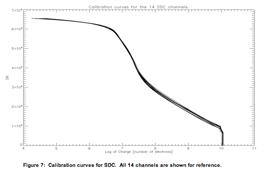 Figure 13-7: Calibration curves for SDC. All 14 channels are shown
for reference.
13.3.2 Calibration - Mass
13.3.2.1 Pre-Flight
The mass can be derived from the charge. It was discovered by
J.A. Simpson and A.J. Tuzzolino that a particle impacting a 28 microns
PVDF film (such as those on SDC) will produce a charge given by
Equation 13-1.
Figure 13-7: Calibration curves for SDC. All 14 channels are shown
for reference.
13.3.2 Calibration - Mass
13.3.2.1 Pre-Flight
The mass can be derived from the charge. It was discovered by
J.A. Simpson and A.J. Tuzzolino that a particle impacting a 28 microns
PVDF film (such as those on SDC) will produce a charge given by
Equation 13-1.
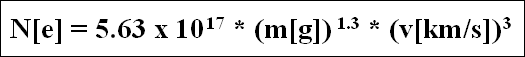 Equation 13-1
In this equation N is the charge in number of electrons, m is the mass in grams, and v is the particle velocity in km/s. On SDC we make one measurement. We can measure the charge produced. Thus to find either mass or velocity we must assume the other. Fortunately the velocity of SDC with respect to the Keplerian orbital velocity of the dust particles is very high. Thus, by assuming that the velocity of the dust is the opposite direction to the velocity of the s/c, the mass can be determined. To verify the results of this equation for our detectors they were taken to the Max Planck Institute in Heidelberg, Germany. With the dust accelerator there, particles of known velocity and mass were accelerated into the detectors and the charge curve produced. From these experiments we were able to verify the curve above with a slightly different constant of 5.63 x 10^17. 13.3.2.2 Mass Production Rearranging the equation above gives Equation 13-2.
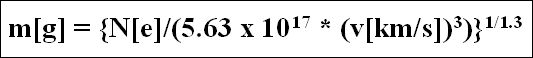 Equation 13-2
Thus one can simply use the number of electrons produced and the velocity of the spacecraft calculated through SPICE to determine the mass of the impacting particle. Note that each event is converted to mass regardless of whether or not it is believed to be noise. 13.4 Calibrated Data Specifics 13.4.1 Algorithm for Pipeline Pre-flight calibration of the electronics box was performed to find the relationship between charge in and DN out. This was done at 4 electronics box temperatures for all 14 channels. Fits were established from this data and the coefficients were stored in a matrix (see Figure 13-7 and section 13.3.1 above). The code for Level 2 data uses the channel number and electronics box temperature to find the correct coefficients in the matrix. These coefficients are then used in a polynomial function, with the raw DN as the independent value, to calculate the corresponding charge, and then converted to mass using the equation the Mass Production equation above. For in-flight box temperatures other than the calibration temperatures represented by the first index of the calibration matrix, the in-flight charge is interpolated (or extrapolated) from the calculated charges using the two nearest calibration temperatures. Finally, in like manner using the standard deviations calibration matrix (SIG), for the nearest DN calibration measurements (DNavg) and nearest two calibration temperatures, as an analog for the 1-sigma combined uncertainty of the calibration charge pulse measurement and of the calibration and in-flight DN measurement, the +/- 1-sigma masses (M_sigplus & M_sigminus) are calculated. 13.4.2 Dataflow Block Diagram
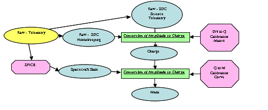 Figure 13-8: Dataflow Block Diagram
13.4.3 Data Format
The calibrated FITS file consists of science data expressed in units
of number of electrons and quality flags for the PVDF detectors. The
quality flags signal whether or not any of the housekeeping values
were out of the standard operating range when the hit occurred. The
quality flags also tell whether or not the data was extrapolated or
interpolated from our pre-flight calibration curve.
Note that for scientific convenience in calibrated data, the channels
are labeled 1-14 instead of 0-13.
13.4.4 Extra FITS Extensions (planes) and Their Definitions
The two tables in the calibrated FITS file are
1) CALIBRATED_DATA -
a. UTC Time
b. MET - Time in Mission Elapsed Time (MET)
c. Channel - [1-14]
d. Charge [Number of Electrons]
e. Mass [grams]
f. Mass_Thrsh - The threshold in mass [grams]
g. M_sigplus - Mass Plus sigma [grams]
h. M_sigminus - Mass Minus sigma [grams]
i. Quality_flag - Because we are susceptible to thruster firings
(i.e. a thruster fire can cause false hits) a flag has been created to
flag events we believe were caused by a thruster..
i. "OK" - No thruster firings occurred near this event
ii. "TF" - A thruster firing occurred within 1 second of this
event and thus we believe the event was possibly caused by a thruster
firing
13.4.5 Scientific Units
Charge - Number of electrons produced from impact.
Mass - Grams of impacting particle.
13.4.6 Additional FITS and PDS Keywords Added
13.4.7 Hardware/OS Development Platform
Intel, Linux or Windows
13.4.8 Language(s) Used
IDL
13.4.9 Third Party Libraries Required
JPL Astro Library downloaded from NASA at Goddard.
13.4.10 Calibration Files Needed (with Quantities)
IDL .sav file consisting of a table for fit coefficients. ( TBD, <1MB
)
13.4.11 Memory Required
TBD
13.4.12 Temporary File System Space Needed
TBD
13.4.13 Predicted Size of Output File(s)
Less than 1KB
13.4.14 Predicted Execution time
A few seconds
13.4.15 Contact/Support Person(s)
Level 1: Andrew Poppe, David James
Level 2: Mihaly Horanyi, David James
13.4.16 Maintenance Schedule (Code/Data Updates, Documentation)
We do have on-board calibration capabilities for the instrument and a
place to insert these changes built into the code. Currently this
simply multiplies by 1, but it the capability to adjust the values by
some specified function remains.
14. SWAP Instrument description
14.1 Overview
Solar Wind Around Pluto (SWAP) instrument is designed to measure the
properties of solar wind ions for the New Horizons mission to Pluto. The
bulk (thermal) solar wind ion distribution is typically Maxwellian. For most
of the long journey to Pluto we expect to encounter bulk solar wind cold ion
distributions that are nearly Maxwellian since the density and temperature
of the solar wind decrease with increasing distance from the Sun,. One
notable exception is when we encounter Jupiter's magnetosheath. Ion
distributions are known to be hot in sheath regions. Since there have been
no prior in situ measurements near Pluto, we do not know if it has a well
developed sheath region.
Figure 13-8: Dataflow Block Diagram
13.4.3 Data Format
The calibrated FITS file consists of science data expressed in units
of number of electrons and quality flags for the PVDF detectors. The
quality flags signal whether or not any of the housekeeping values
were out of the standard operating range when the hit occurred. The
quality flags also tell whether or not the data was extrapolated or
interpolated from our pre-flight calibration curve.
Note that for scientific convenience in calibrated data, the channels
are labeled 1-14 instead of 0-13.
13.4.4 Extra FITS Extensions (planes) and Their Definitions
The two tables in the calibrated FITS file are
1) CALIBRATED_DATA -
a. UTC Time
b. MET - Time in Mission Elapsed Time (MET)
c. Channel - [1-14]
d. Charge [Number of Electrons]
e. Mass [grams]
f. Mass_Thrsh - The threshold in mass [grams]
g. M_sigplus - Mass Plus sigma [grams]
h. M_sigminus - Mass Minus sigma [grams]
i. Quality_flag - Because we are susceptible to thruster firings
(i.e. a thruster fire can cause false hits) a flag has been created to
flag events we believe were caused by a thruster..
i. "OK" - No thruster firings occurred near this event
ii. "TF" - A thruster firing occurred within 1 second of this
event and thus we believe the event was possibly caused by a thruster
firing
13.4.5 Scientific Units
Charge - Number of electrons produced from impact.
Mass - Grams of impacting particle.
13.4.6 Additional FITS and PDS Keywords Added
13.4.7 Hardware/OS Development Platform
Intel, Linux or Windows
13.4.8 Language(s) Used
IDL
13.4.9 Third Party Libraries Required
JPL Astro Library downloaded from NASA at Goddard.
13.4.10 Calibration Files Needed (with Quantities)
IDL .sav file consisting of a table for fit coefficients. ( TBD, <1MB
)
13.4.11 Memory Required
TBD
13.4.12 Temporary File System Space Needed
TBD
13.4.13 Predicted Size of Output File(s)
Less than 1KB
13.4.14 Predicted Execution time
A few seconds
13.4.15 Contact/Support Person(s)
Level 1: Andrew Poppe, David James
Level 2: Mihaly Horanyi, David James
13.4.16 Maintenance Schedule (Code/Data Updates, Documentation)
We do have on-board calibration capabilities for the instrument and a
place to insert these changes built into the code. Currently this
simply multiplies by 1, but it the capability to adjust the values by
some specified function remains.
14. SWAP Instrument description
14.1 Overview
Solar Wind Around Pluto (SWAP) instrument is designed to measure the
properties of solar wind ions for the New Horizons mission to Pluto. The
bulk (thermal) solar wind ion distribution is typically Maxwellian. For most
of the long journey to Pluto we expect to encounter bulk solar wind cold ion
distributions that are nearly Maxwellian since the density and temperature
of the solar wind decrease with increasing distance from the Sun,. One
notable exception is when we encounter Jupiter's magnetosheath. Ion
distributions are known to be hot in sheath regions. Since there have been
no prior in situ measurements near Pluto, we do not know if it has a well
developed sheath region.
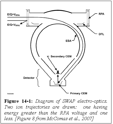 Figure 14-1: Diagram of SWAP electro-optics. Two ion trajectories are
drawn: one having energy greater than the RPA voltage and one less. [Figure
8 from McComas et al., 2007]
The SWAP instrument is an electrostatic instrument. The SWAP electro-optics
control the energy passband of ions entering the instrument. The
electro-optics has three parts: the Retarding Potential Analyzer (RPA), the
Electrostatic Analyzer (ESA), and the deflector (DFL). Figure 14-1 shows a
cross section of the instrument. The RPA consists of four grids with the
inner two having a positive voltage, which repels ions with energies less
than the corresponding potential energy (qV) (top right and left of Figure
14-1). The Electrostatic Analyzer has two parts, which are concentrically
spaced, an inner dome and an outer spherical shell (at ground). Only ions
with a limited range of energies pass through the ESA to reach the detector.
The SWAP instrument is mounted on the -Zsc side of the spacecraft and
the normal to the center of the aperture is aligned with +Ysc (Figure
14-2). Figure 14-3 shows the instrument being mounted to the spacecraft.
The deflector is used to adjust the field of view. That is if the solar
wind, which is highly collimated (spanning only a few degrees), enters at
the bottom of the RPA, the voltage on the deflector could be set so that
only ions that are not part of the solar wind beam enter the instrument.
This would allow pickup ions, which occur over a wide range of angles, to be
studied. In the inner heliosphere the pickup ions have substantially lower
fluxes than the solar wind. The SWAP deflector can be used to bring the
solar wind into the field of view if the solar wind beam is slightly above
the top of the nominal field of view. Operating the deflector affects the
energy of the ions that can enter the ESA. The RPA voltage is adjusted to
compensate such that the same energy ions enter the ESA as did prior to the
deflector voltage change. The deflector voltage can be automatically varied
based on the commanded angle. The voltage settings for the ESA, RPA,
deflector, and the amount the RPA should be adjusted to compensate for the
deflector setting are all specified using lookup tables, which allow many
instrument operation changes to be made by uploading new tables without
having to make any software changes. Additional information on the
electro-optical design is given in the introduction of section 3 and in
section 3.1 in the McComas et al. [2007] instrument paper. The CEM detector
design is also described in section 3.1.
Figure 14-1: Diagram of SWAP electro-optics. Two ion trajectories are
drawn: one having energy greater than the RPA voltage and one less. [Figure
8 from McComas et al., 2007]
The SWAP instrument is an electrostatic instrument. The SWAP electro-optics
control the energy passband of ions entering the instrument. The
electro-optics has three parts: the Retarding Potential Analyzer (RPA), the
Electrostatic Analyzer (ESA), and the deflector (DFL). Figure 14-1 shows a
cross section of the instrument. The RPA consists of four grids with the
inner two having a positive voltage, which repels ions with energies less
than the corresponding potential energy (qV) (top right and left of Figure
14-1). The Electrostatic Analyzer has two parts, which are concentrically
spaced, an inner dome and an outer spherical shell (at ground). Only ions
with a limited range of energies pass through the ESA to reach the detector.
The SWAP instrument is mounted on the -Zsc side of the spacecraft and
the normal to the center of the aperture is aligned with +Ysc (Figure
14-2). Figure 14-3 shows the instrument being mounted to the spacecraft.
The deflector is used to adjust the field of view. That is if the solar
wind, which is highly collimated (spanning only a few degrees), enters at
the bottom of the RPA, the voltage on the deflector could be set so that
only ions that are not part of the solar wind beam enter the instrument.
This would allow pickup ions, which occur over a wide range of angles, to be
studied. In the inner heliosphere the pickup ions have substantially lower
fluxes than the solar wind. The SWAP deflector can be used to bring the
solar wind into the field of view if the solar wind beam is slightly above
the top of the nominal field of view. Operating the deflector affects the
energy of the ions that can enter the ESA. The RPA voltage is adjusted to
compensate such that the same energy ions enter the ESA as did prior to the
deflector voltage change. The deflector voltage can be automatically varied
based on the commanded angle. The voltage settings for the ESA, RPA,
deflector, and the amount the RPA should be adjusted to compensate for the
deflector setting are all specified using lookup tables, which allow many
instrument operation changes to be made by uploading new tables without
having to make any software changes. Additional information on the
electro-optical design is given in the introduction of section 3 and in
section 3.1 in the McComas et al. [2007] instrument paper. The CEM detector
design is also described in section 3.1.
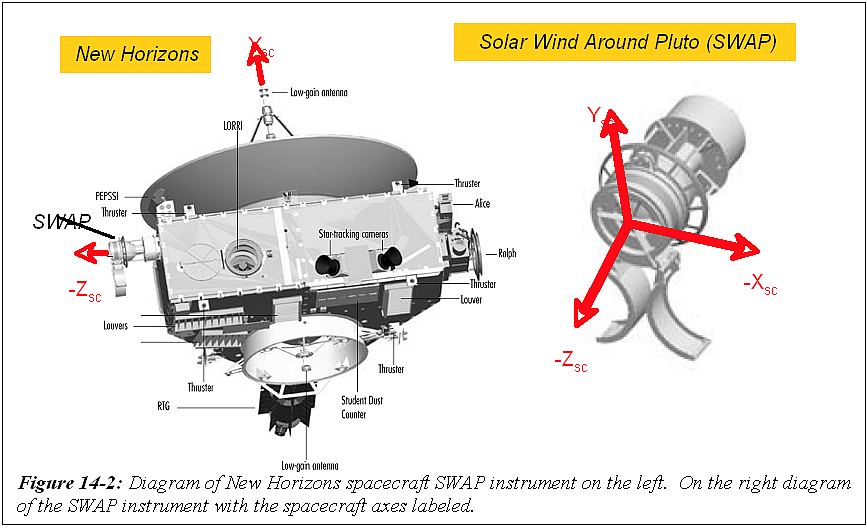 Figure 14-2: Diagram of New Horizons spacecraft SWAP instrument on the
left. On the right diagram of the SWAP instrument with the spacecraft axes
labeled.
The SWAP instrument has two kinds of voltage scans (also called sweeps):
coarse and fine. The voltage settings are predefined with onboard voltage
tables. In coarse scans large voltage steps are taken with the ESA and RPA
holding the ratio of the two voltages fixed. In the fine scans we also hold
the RPA and ESA at constant ratio, but take smaller steps. Our voltage
tables allow us to vary the ratio between the RPA and ESA voltages, but
typically this ratio is held constant as much as possible. For high ESA
voltages we cannot set the RPA to a high enough voltage to keep the RPA and
ESA voltage ratio fixed because the highest RPA voltage is 2000 V and the
highest ESA voltage is 4000 V. A given step number refers to a pair of RPA
and ESA voltages. In the inner heliosphere we set the RPA to ESA voltage
ratio high in order to narrow the passband slightly by removing ions at the
low energies. All fine scans are approximately centered about the step
number where the peak counts are observed in the coarse scan. To determine
plasma properties from the detected count rates as a function of step
number, the following calibration information is necessary: the ESA and RPA
response functions, angular response function, the instrument solid angle,
the detector gain, and the effective area.
Onboard there is one ESA table with 1024 steps and 4 RPA tables with 1024
steps each. For a given sweep we use the ESA table and one of the RPA
tables. The different RPA tables can be used for coarse and fine scans, but
currently for Jupiter operations we are using the same RPA table for both
the coarse and fine scans. In a scan/sweep the same step number is used in
the software to reference rows in the ESA table and the chosen RPA table.
The coarse scans use every 16th step in the 1024 step table where a step
refers to a RPA and ESA voltage pairing. A fine scan consists of 64 steps
with the coarse step at which the peak counts were detected in the middle of
the fine scan (16*64=1024).
Figure 14-2: Diagram of New Horizons spacecraft SWAP instrument on the
left. On the right diagram of the SWAP instrument with the spacecraft axes
labeled.
The SWAP instrument has two kinds of voltage scans (also called sweeps):
coarse and fine. The voltage settings are predefined with onboard voltage
tables. In coarse scans large voltage steps are taken with the ESA and RPA
holding the ratio of the two voltages fixed. In the fine scans we also hold
the RPA and ESA at constant ratio, but take smaller steps. Our voltage
tables allow us to vary the ratio between the RPA and ESA voltages, but
typically this ratio is held constant as much as possible. For high ESA
voltages we cannot set the RPA to a high enough voltage to keep the RPA and
ESA voltage ratio fixed because the highest RPA voltage is 2000 V and the
highest ESA voltage is 4000 V. A given step number refers to a pair of RPA
and ESA voltages. In the inner heliosphere we set the RPA to ESA voltage
ratio high in order to narrow the passband slightly by removing ions at the
low energies. All fine scans are approximately centered about the step
number where the peak counts are observed in the coarse scan. To determine
plasma properties from the detected count rates as a function of step
number, the following calibration information is necessary: the ESA and RPA
response functions, angular response function, the instrument solid angle,
the detector gain, and the effective area.
Onboard there is one ESA table with 1024 steps and 4 RPA tables with 1024
steps each. For a given sweep we use the ESA table and one of the RPA
tables. The different RPA tables can be used for coarse and fine scans, but
currently for Jupiter operations we are using the same RPA table for both
the coarse and fine scans. In a scan/sweep the same step number is used in
the software to reference rows in the ESA table and the chosen RPA table.
The coarse scans use every 16th step in the 1024 step table where a step
refers to a RPA and ESA voltage pairing. A fine scan consists of 64 steps
with the coarse step at which the peak counts were detected in the middle of
the fine scan (16*64=1024).
 Figure 14-3: Picture of SWAP being mounted to the spacecraft.
14.2 Electronics and Flight Software
The instrument electronics are described in section 3.4 of the McComas et
al. [2007] instrument paper. In subsequent sections of this document some
information related to the flight software is provided, but further details
are provided in sections 3.6 of the instrument paper.
14.3 SWAP Data Types
There are six types of SWAP science and engineering data: real-time science
(0x584), summary (0x585), histogram (0x586), housekeeping, messages, and
memory dump. Housekeeping, messages, and memory dump provide engineering
data and the other three modes contain science data. Real-time data provide
the most detailed science measurements since they contain the full count
rate distribution as a function of energy (speed). For science summary and
science histogram modes, the full distribution is not recorded. Instead,
parameters are derived from the count rate distribution stored by SWAP.
These derived parameters require less memory than storing the whole
distribution. The science summary and science histogram modes are primarily
used during the cruise phase of the mission.
The real-time science data contain the full count rate energy distribution
for the primary, secondary and coincidence rates. The full distribution is
desired because in bow shock and sheath regions plasma distributions may not
be Maxwellian. The shape of the distribution will provide valuable
information about what physical processes are occurring. In real-time mode
the instrument can take measurements at a rate of 1 Hz, which is crucial for
studying plasma boundaries and shocks.
Summary data consist of parameters related to the average speed,
temperature, and density. The summary data are designed to study the bulk
solar wind. The peak of the count distribution is related to the density,
the bin location of the peak is related to the speed, and the distribution
width is related to the temperature and speed combined. Along with the
average values, the variance, maximum and minimum values of the peak counts,
width of the peak, and energy of the peak are also recorded.
The histogram data are designed to study pickup ions. The pickup ion
distribution has a characteristic shape once it is normalized by the average
solar wind energy (or speed). The histogram data conserve storage space by
adding up all the counts detected in given bins. The accumulation time for
the histogram is variable. The bins for the histograms are not energy bins,
but are bins relative the average solar wind energy (Esw). The steps for the
fine scan are roughly centered on the coarse scan step where the peak counts
were observed allowing the energy of the solar wind to be more precisely
determined in the fine scan. The energy found in the fine scan is then used
to place the counts determined in the coarse ESA scan into a new large 1-D
histogram array. The coarse scan count rate data array is placed into the
larger histogram array such that the bin with the maximum counts in the fine
scan is placed into histogram bin 1024. There are 1024 possible voltages in
a given onboard voltage table. To understand the histogram data further
information about the scans is necessary. Onboard there is one ESA table
with 1024 steps and 4 RPA tables with 1024 steps each. For a given sweep we
use the ESA table and one of the RPA tables. The different RPA tables can be
used for coarse and fine scans, but currently for Jupiter operations we are
using the same RPA table for both the coarse and fine scans. In a scan/sweep
the same step number is used in the software to reference rows in the ESA
table and the chosen RPA table. The coarse scans use every 16th step in the
1024 step table where a step refers to a RPA and ESA voltage pairing. A fine
scan consists of 64 steps with the coarse step at which the peak counts were
detected in the middle of the fine scan (16*64=1024). There are 2048 bins
because the peak count rate in a fine scan could occur at any step in the
fine scan, and the step in the coarse scan containing the peak counts is
always place in bin 1024.
When another set of coarse-fine scans is performed, the new array of counts
is processed in a similar fashion. The new data are placed into bins such
that the new peak counts aligned with bin 1024, and then added to the
running total number of counts. The amount of data put into each histogram
bin is tracked in a separate array. The histogram packets then consist of
two 1-D vectors: one for counts in the bins and one for the number of
samples placed into each bin (Example shown in Figure 14-4 ).
Figure 14-3: Picture of SWAP being mounted to the spacecraft.
14.2 Electronics and Flight Software
The instrument electronics are described in section 3.4 of the McComas et
al. [2007] instrument paper. In subsequent sections of this document some
information related to the flight software is provided, but further details
are provided in sections 3.6 of the instrument paper.
14.3 SWAP Data Types
There are six types of SWAP science and engineering data: real-time science
(0x584), summary (0x585), histogram (0x586), housekeeping, messages, and
memory dump. Housekeeping, messages, and memory dump provide engineering
data and the other three modes contain science data. Real-time data provide
the most detailed science measurements since they contain the full count
rate distribution as a function of energy (speed). For science summary and
science histogram modes, the full distribution is not recorded. Instead,
parameters are derived from the count rate distribution stored by SWAP.
These derived parameters require less memory than storing the whole
distribution. The science summary and science histogram modes are primarily
used during the cruise phase of the mission.
The real-time science data contain the full count rate energy distribution
for the primary, secondary and coincidence rates. The full distribution is
desired because in bow shock and sheath regions plasma distributions may not
be Maxwellian. The shape of the distribution will provide valuable
information about what physical processes are occurring. In real-time mode
the instrument can take measurements at a rate of 1 Hz, which is crucial for
studying plasma boundaries and shocks.
Summary data consist of parameters related to the average speed,
temperature, and density. The summary data are designed to study the bulk
solar wind. The peak of the count distribution is related to the density,
the bin location of the peak is related to the speed, and the distribution
width is related to the temperature and speed combined. Along with the
average values, the variance, maximum and minimum values of the peak counts,
width of the peak, and energy of the peak are also recorded.
The histogram data are designed to study pickup ions. The pickup ion
distribution has a characteristic shape once it is normalized by the average
solar wind energy (or speed). The histogram data conserve storage space by
adding up all the counts detected in given bins. The accumulation time for
the histogram is variable. The bins for the histograms are not energy bins,
but are bins relative the average solar wind energy (Esw). The steps for the
fine scan are roughly centered on the coarse scan step where the peak counts
were observed allowing the energy of the solar wind to be more precisely
determined in the fine scan. The energy found in the fine scan is then used
to place the counts determined in the coarse ESA scan into a new large 1-D
histogram array. The coarse scan count rate data array is placed into the
larger histogram array such that the bin with the maximum counts in the fine
scan is placed into histogram bin 1024. There are 1024 possible voltages in
a given onboard voltage table. To understand the histogram data further
information about the scans is necessary. Onboard there is one ESA table
with 1024 steps and 4 RPA tables with 1024 steps each. For a given sweep we
use the ESA table and one of the RPA tables. The different RPA tables can be
used for coarse and fine scans, but currently for Jupiter operations we are
using the same RPA table for both the coarse and fine scans. In a scan/sweep
the same step number is used in the software to reference rows in the ESA
table and the chosen RPA table. The coarse scans use every 16th step in the
1024 step table where a step refers to a RPA and ESA voltage pairing. A fine
scan consists of 64 steps with the coarse step at which the peak counts were
detected in the middle of the fine scan (16*64=1024). There are 2048 bins
because the peak count rate in a fine scan could occur at any step in the
fine scan, and the step in the coarse scan containing the peak counts is
always place in bin 1024.
When another set of coarse-fine scans is performed, the new array of counts
is processed in a similar fashion. The new data are placed into bins such
that the new peak counts aligned with bin 1024, and then added to the
running total number of counts. The amount of data put into each histogram
bin is tracked in a separate array. The histogram packets then consist of
two 1-D vectors: one for counts in the bins and one for the number of
samples placed into each bin (Example shown in Figure 14-4 ).
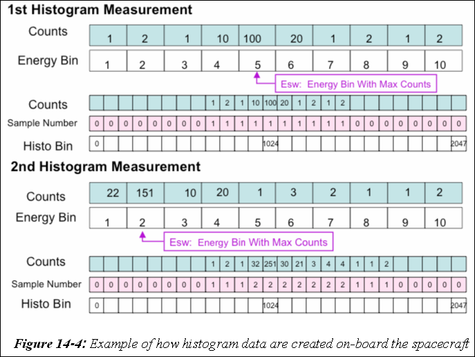 Figure 14-4: Example of how histogram data are created on-board the
spacecraft
The histogram data consist of a series of 64 packets to facilitate data
transmission. There are two types of histogram packets. For each histogram
type 1 packet, there should be 63 histogram type 2 packets. One type 1 and
63 type 2 histogram packets are combined when placed into the Level 2 (raw)
files. The histogram type 1 packets contain information about the data
collection such as the start and end time of the data collection interval
and the plan and sweep numbers. Type 1 contains a small portion of the
histogram data, but most of the histogram data is contained in the Type 2
packets, which hold a larger amount of data since they do not contain
information about the data collection.
14.4 Raw File (Level 2) Specifics
14.4.1 Data Format
Figure 14-4: Example of how histogram data are created on-board the
spacecraft
The histogram data consist of a series of 64 packets to facilitate data
transmission. There are two types of histogram packets. For each histogram
type 1 packet, there should be 63 histogram type 2 packets. One type 1 and
63 type 2 histogram packets are combined when placed into the Level 2 (raw)
files. The histogram type 1 packets contain information about the data
collection such as the start and end time of the data collection interval
and the plan and sweep numbers. Type 1 contains a small portion of the
histogram data, but most of the histogram data is contained in the Type 2
packets, which hold a larger amount of data since they do not contain
information about the data collection.
14.4 Raw File (Level 2) Specifics
14.4.1 Data Format
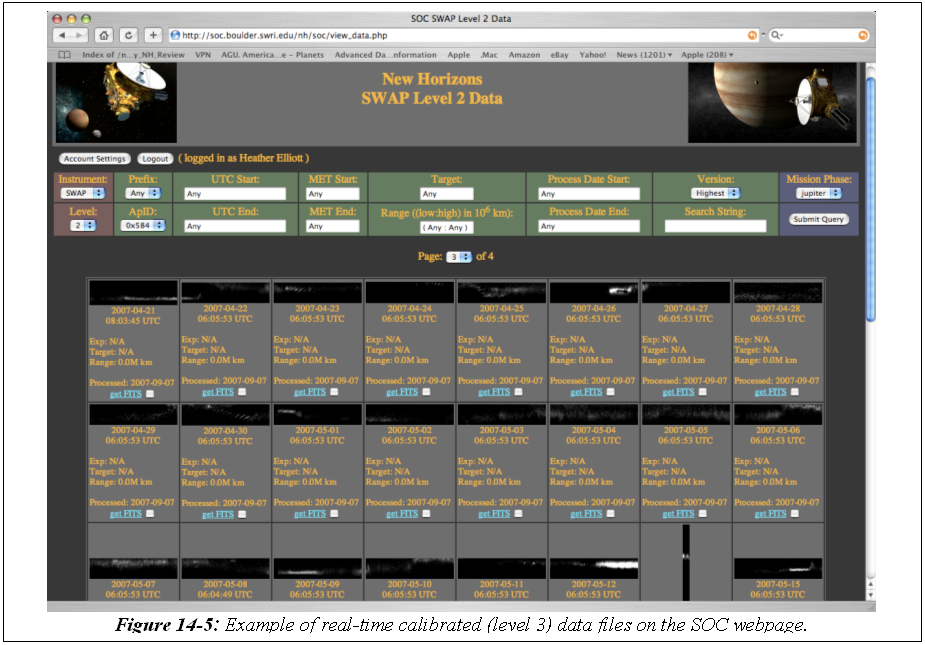 Figure 14-5: Example of real-time calibrated (level 3) data files on the
SOC webpage.
There are separate files for summary, histogram, and real-time data, and
corresponding housekeeping data are placed in each file. Note that not all
kinds of packets will be generated every day. For example, during
commissioning there may only be housekeeping and memory dump packets, and
during cruise there will be housekeeping, summary, and histogram packets.
All the packet types have a CHKSUM parameter. This parameter is calculated
onboard and is also calculated on the ground to check the data. In Figure
14-5 we show what the calibrated files look like on the SOC web site. For
the real-time data there are black and white images of the coincidence
spectrogram array where the y-axis is energy bin number and the x-axis is
time bin number.
Real-time science packets can occur at a rate as high as 1 Hz where each
packet contains a set of counts, voltages, etc. A set of two observations
are stored in one packet. One observation occurs in the 1st half second and
a 2nd observation occurs in the 2nd half second. The 1st and 2nd half second
measurements correspond to two different steps in a given sweep. Each step
consists of an RPA and ESA voltage pairing, and 64 such pairs complete
either a coarse-coarse scan or a coarse-fine scan. In a coarse-coarse scan
two 64 step (32 packets) coarse scans are done back to back. In a
coarse-fine scan a 64 step (32 packets) coarse scan and then a 64 step (32
packets) fine is performed. Both a complete coarse-coarse, and a coarse-fine
scan have 64 packets. There is a parameter called SWAP_RT.sec64_ST, which is
included in every real-time science packet and has the value 1 at the start
of a pair of scans (a set of 64 packets) and is zero otherwise. We use this
parameter to insure that a 64 second cycle (pair of scans) is not split
across a day.
The SWAP raw (level 2) data are arranged in a binary table such that the
columns are instrument parameters and measurements, and rows are measurement
times. The FITS format has a binary table that allows for columns and rows.
Below in Figure 14-6 is a picture of what the Level 2 raw real-time files
look like using FITS Viewer (FV). As mentioned earlier the housekeeping data
are also in an table extension. The histogram counts and number of samples
are stored as image extensions. The zeroth extension contains only the
primary header, the first extension holds the real-time data, the second
extension holds the housekeeping data, and the third extension holds the
thruster data.
Figure 14-5: Example of real-time calibrated (level 3) data files on the
SOC webpage.
There are separate files for summary, histogram, and real-time data, and
corresponding housekeeping data are placed in each file. Note that not all
kinds of packets will be generated every day. For example, during
commissioning there may only be housekeeping and memory dump packets, and
during cruise there will be housekeeping, summary, and histogram packets.
All the packet types have a CHKSUM parameter. This parameter is calculated
onboard and is also calculated on the ground to check the data. In Figure
14-5 we show what the calibrated files look like on the SOC web site. For
the real-time data there are black and white images of the coincidence
spectrogram array where the y-axis is energy bin number and the x-axis is
time bin number.
Real-time science packets can occur at a rate as high as 1 Hz where each
packet contains a set of counts, voltages, etc. A set of two observations
are stored in one packet. One observation occurs in the 1st half second and
a 2nd observation occurs in the 2nd half second. The 1st and 2nd half second
measurements correspond to two different steps in a given sweep. Each step
consists of an RPA and ESA voltage pairing, and 64 such pairs complete
either a coarse-coarse scan or a coarse-fine scan. In a coarse-coarse scan
two 64 step (32 packets) coarse scans are done back to back. In a
coarse-fine scan a 64 step (32 packets) coarse scan and then a 64 step (32
packets) fine is performed. Both a complete coarse-coarse, and a coarse-fine
scan have 64 packets. There is a parameter called SWAP_RT.sec64_ST, which is
included in every real-time science packet and has the value 1 at the start
of a pair of scans (a set of 64 packets) and is zero otherwise. We use this
parameter to insure that a 64 second cycle (pair of scans) is not split
across a day.
The SWAP raw (level 2) data are arranged in a binary table such that the
columns are instrument parameters and measurements, and rows are measurement
times. The FITS format has a binary table that allows for columns and rows.
Below in Figure 14-6 is a picture of what the Level 2 raw real-time files
look like using FITS Viewer (FV). As mentioned earlier the housekeeping data
are also in an table extension. The histogram counts and number of samples
are stored as image extensions. The zeroth extension contains only the
primary header, the first extension holds the real-time data, the second
extension holds the housekeeping data, and the third extension holds the
thruster data.
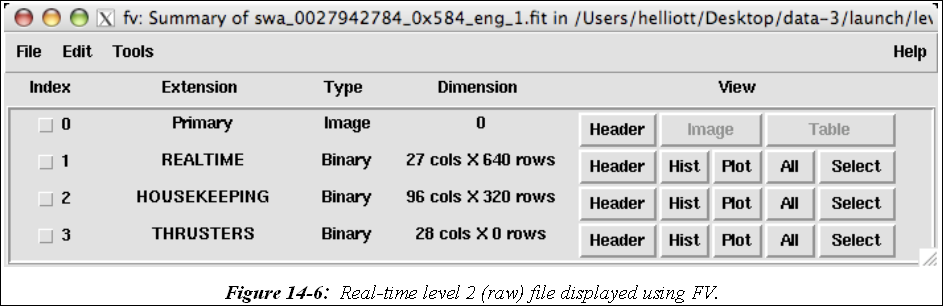 Figure 14-6: Real-time level 2 (raw) file displayed using FV.
SWAP data are in CCSDS packets packetized by the spacecraft from the
low-speed bus. Note that on the New Horizons mission, every instrument also
outputs a non-packetized portion of telemetry to the S/C. This portion is
also called the instrument state and this data is incorporated into the
general spacecraft housekeeping data and not into the SWAP packets. All the
bits in the SWAP packets were defined for the MOC at APL in EXCEL
spreadsheets in the form required by the mission. The New Horizons SOC used
the same bit level format description (APL EXCEL spreadsheets) for all the
parameters in our packets to decode our raw (level 2) data.
14.4.2 Definition of an Observation
A complete histogram observation consists of one histogram type 1 packet and
63 histogram type 2 packets. A complete set of real-time science
measurements consists of a full 64-second cycle. This is described in detail
in section 14.4.1. One summary packet constitutes a complete measurement.
Housekeeping data are required for all science measurements since the
housekeeping data are key to interpreting the data and determining error
flags.
14.4.3 Housekeeping Needed in Level 2(Raw) Files (for Calibration)
Unlike some of the other instruments all housekeeping data for SWAP are
included into the level 2 (raw) files as an extension.
14.4.4 Raw Science Data and/or Housekeeping Requirements
In addition to the complete housekeeping packets, raw summary, real-time,
histogram, and thruster fire packets are included into our raw (level 2)
files. The thruster data format for the raw files was reformatted to reduce
space (Joe Peterson). In the calibrated (level 3) data the thruster data
has been arranged by thruster name and time. The numbers in the table
indicate the duration of the thruster firings.
Figure 14-6: Real-time level 2 (raw) file displayed using FV.
SWAP data are in CCSDS packets packetized by the spacecraft from the
low-speed bus. Note that on the New Horizons mission, every instrument also
outputs a non-packetized portion of telemetry to the S/C. This portion is
also called the instrument state and this data is incorporated into the
general spacecraft housekeeping data and not into the SWAP packets. All the
bits in the SWAP packets were defined for the MOC at APL in EXCEL
spreadsheets in the form required by the mission. The New Horizons SOC used
the same bit level format description (APL EXCEL spreadsheets) for all the
parameters in our packets to decode our raw (level 2) data.
14.4.2 Definition of an Observation
A complete histogram observation consists of one histogram type 1 packet and
63 histogram type 2 packets. A complete set of real-time science
measurements consists of a full 64-second cycle. This is described in detail
in section 14.4.1. One summary packet constitutes a complete measurement.
Housekeeping data are required for all science measurements since the
housekeeping data are key to interpreting the data and determining error
flags.
14.4.3 Housekeeping Needed in Level 2(Raw) Files (for Calibration)
Unlike some of the other instruments all housekeeping data for SWAP are
included into the level 2 (raw) files as an extension.
14.4.4 Raw Science Data and/or Housekeeping Requirements
In addition to the complete housekeeping packets, raw summary, real-time,
histogram, and thruster fire packets are included into our raw (level 2)
files. The thruster data format for the raw files was reformatted to reduce
space (Joe Peterson). In the calibrated (level 3) data the thruster data
has been arranged by thruster name and time. The numbers in the table
indicate the duration of the thruster firings.
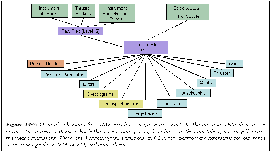 Figure 14-7: General Schematic for SWAP Pipeline. In green are inputs to
the pipeline. Data files are in purple. The primary extension holds the main
header (orange). In blue are the data tables, and in yellow are the image
extensions.There are 3 spectrogram extensions and 3 error spectrogram
extensions for our three count rate signals: PCEM, SCEM, and coincidence.
14.5 Calibrated (Level 3) File Specifics
14.5.1 Data Format
The SWAP calibrated (level 3) pipeline requires the following input
information, SWAP level 2 (raw) files which include all the housekeeping
data, SWAP calibration information and engineering factors, orbit and
attitude information, and spacecraft information such as thruster firings.
In Figure 14-7 we show a general schematic for our level 3 (calibrated)
real-time data files. The main input to the calibration pipeline are the
SPICE kernels, and raw level 2 files which include the real-time data,
thruster firings, a few minor calculations performed using SPICE in the
header and the housekeeping data..
The SWAP level 3 (calibrated) analysis software has four parts corresponding
to the different data (packet) types. There are simple algorithms for
converting the raw data to engineering units. For example in the raw data
the RPA voltage is stored as a step number for the Digital to Analog
Converter (DAC), and not the actual voltage. We first make all such
engineering conversions. Most information in our calibrated (level 3) files
is stored in table format (blue blocks in diagram). The tables contain all
the data (science and housekeeping) converted to engineering units, and
counts are converted to count rate (Hz). There are extensions for
housekeeping data, thruster firing data, and quality flags. In the real-time
data there are additional image extensions for spectrograms derived from
high voltage science real-time measurements. There are three count rate 2-D
arrays for the SCEM, PCEM, and coincidence signals stored as images, and
three corresponding count rate error image extensions. These errors will be
based on counting statistics. In addition to the 2-D arrays, axis
information is also necessary for the spectrograms. The axis information for
the spectrograms are contained in two tables one with the energy per charge
(E/q) and one with the time tags fore each sweep. In Figure 14-8 we show a
picture of what the real-time files look like when opened using the FITS
viewer FV.
Figure 14-7: General Schematic for SWAP Pipeline. In green are inputs to
the pipeline. Data files are in purple. The primary extension holds the main
header (orange). In blue are the data tables, and in yellow are the image
extensions.There are 3 spectrogram extensions and 3 error spectrogram
extensions for our three count rate signals: PCEM, SCEM, and coincidence.
14.5 Calibrated (Level 3) File Specifics
14.5.1 Data Format
The SWAP calibrated (level 3) pipeline requires the following input
information, SWAP level 2 (raw) files which include all the housekeeping
data, SWAP calibration information and engineering factors, orbit and
attitude information, and spacecraft information such as thruster firings.
In Figure 14-7 we show a general schematic for our level 3 (calibrated)
real-time data files. The main input to the calibration pipeline are the
SPICE kernels, and raw level 2 files which include the real-time data,
thruster firings, a few minor calculations performed using SPICE in the
header and the housekeeping data..
The SWAP level 3 (calibrated) analysis software has four parts corresponding
to the different data (packet) types. There are simple algorithms for
converting the raw data to engineering units. For example in the raw data
the RPA voltage is stored as a step number for the Digital to Analog
Converter (DAC), and not the actual voltage. We first make all such
engineering conversions. Most information in our calibrated (level 3) files
is stored in table format (blue blocks in diagram). The tables contain all
the data (science and housekeeping) converted to engineering units, and
counts are converted to count rate (Hz). There are extensions for
housekeeping data, thruster firing data, and quality flags. In the real-time
data there are additional image extensions for spectrograms derived from
high voltage science real-time measurements. There are three count rate 2-D
arrays for the SCEM, PCEM, and coincidence signals stored as images, and
three corresponding count rate error image extensions. These errors will be
based on counting statistics. In addition to the 2-D arrays, axis
information is also necessary for the spectrograms. The axis information for
the spectrograms are contained in two tables one with the energy per charge
(E/q) and one with the time tags fore each sweep. In Figure 14-8 we show a
picture of what the real-time files look like when opened using the FITS
viewer FV.
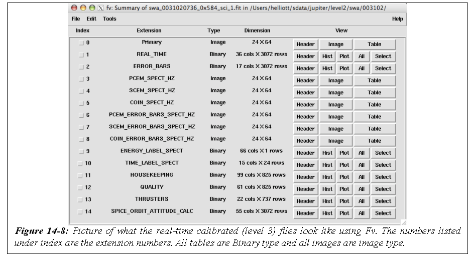 Figure 14-8: Picture of what the real-time calibrated (level 3) files look
like using Fv. The numvers listed under index are the extension numbers. All
tables are Binary type and all images are image type.
14.5.2 Further Algorithm details for Pipeline
In this section we describe the algorithm for SWAP level 3 (calibrated)
processing. As mentioned above The first step in our processing is to
convert all raw values over to engineering units. These conversion factors
are also stored in the command and telemetry spreadsheets used in the APL
GSEOS system. The details of the housekeeping processing are not discussed
further since processing of the housekeeping data consists of simple
conversion factors. Analysis of ground calibration data provides critical
information used to process the SWAP data, and is consequently a crucial
input to our software. A description of the type of calibration information
used in the pipeline is given in the calibration document.
14.5.3 Real-time science data processing
Figure 14-8: Picture of what the real-time calibrated (level 3) files look
like using Fv. The numvers listed under index are the extension numbers. All
tables are Binary type and all images are image type.
14.5.2 Further Algorithm details for Pipeline
In this section we describe the algorithm for SWAP level 3 (calibrated)
processing. As mentioned above The first step in our processing is to
convert all raw values over to engineering units. These conversion factors
are also stored in the command and telemetry spreadsheets used in the APL
GSEOS system. The details of the housekeeping processing are not discussed
further since processing of the housekeeping data consists of simple
conversion factors. Analysis of ground calibration data provides critical
information used to process the SWAP data, and is consequently a crucial
input to our software. A description of the type of calibration information
used in the pipeline is given in the calibration document.
14.5.3 Real-time science data processing
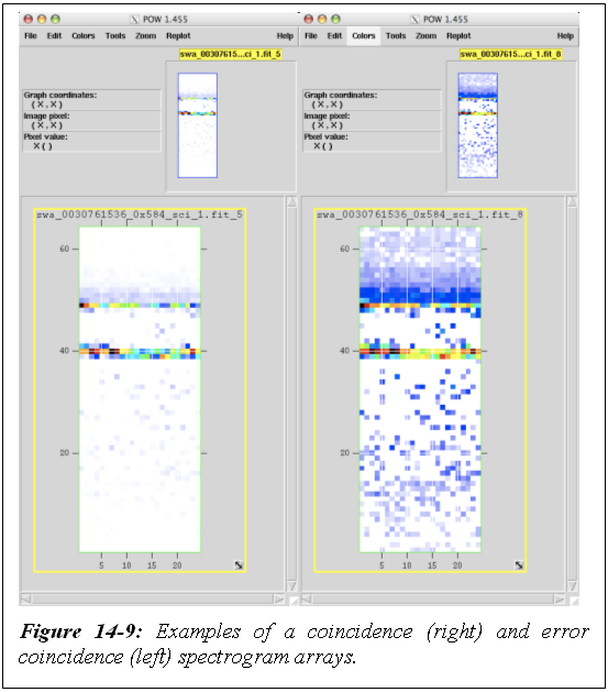 Figure 14-9: Examples of a coincidence (right) and error coincidence (left)
spectrogram arrays.
The identifier in the SOC filenames for real-time data is the APID 0x584.
Our real-time high voltage science (HVSCI) analysis begins by determining
the count rates in Hz as a function of energy for each measurement. A
spectrogram is created by sorting the data into sweeps in order to build a
2-D array where the y-axis is energy per charge and the x-axis is time. A
spectrogram spans the time range in HVSCI mode in a given daily level 2
(raw) file. Spectrograms are created for each of the 3 count signals (PCEM,
SCEM, and coincidence). Corresponding count rate error spectrograms are
created based on counting statistics for each of the three signals as
described in the next paragraph. The x-axis time information is provided in
the TIME_LABEL_SPECT extension along with a column indicating if a
background has been removed. The background is mentioned in section 14.5.10
and described in detail in the calibration document. Also in the
TIME_LABEL_SPECT extension is a column indicating the plan and sweep used
since the energy bins are different for different plans and sweeps. The
y-axis energy labels for a given sweep and plan number are provided in the
ENERGY_LABEL_SPECT extension. These count rate spectrograms provide a way to
examine our data at high time resolution over the full energy range of the
instrument. These kinds of spectrograms have proven useful for analyzing
high time resolution plasma in situ measurements. Having a high time
resolution product is critical for identifying plasma boundaries and shocks.
In Figure 14-9 we show examples of what coincidence and an error coincidence
spectrogram arrays look like when opened in FV.
14.5.4 Errors
In the level 3 (calibrated) data files an error value for every measurement
is given in the extension labeled ERROR_BARS. We also provide spectrogram
arrays for each signal type for the errors in the extensions labeled
X_ERROR_BARS_SPECT_HZ where X is PCEM, SCEM, or COIN. The errors provided
are errors for the rates. The errors and include an error for the sample
time, and data compression when compression occurs. The raw rate (count
counts per sample (C)) are convert to Hz using the 0.390 sec
sample/accumulation time (t) (Equation 1). The error squared is given in
Equations 2 and 3, and the fractional error squared is shown Equation 4.
Taking the square root the resulting fractional error is given by equation
5. The final error given in the data files is shown in Equation 6. If the
count rates are not compressed (Cuncomp) then C = Cuncomp and deltaC =
(Cuncomp)^(1/2). However, if the counts are compressed (Ccomp) then C =
16Ccomp + 7.5 and deltaC=(16Ccomp + 7.5)^(1/2). In the ERROR table there
is a column indicating if a background has been removed. The background is
mentioned section 14.5.10 and described in detail in the calibration
document.
C
Rc = - (Equation 1)
t
2 2
2 /dRc\ 2 /dRc\ 2
(deltaRc) = ( --- ) (deltat) + ( --- ) (deltaC) (Equation 2)
\dt / \dt /
N.B. d prefix implies partial derivative
in Equation 2
2 2
2 C 2 /1\ 2
(deltaRc) = -- (deltat) + ( - ) (deltaC) (Equation 3)
4 \t/
t
2 2 2
(deltaRc) (deltat) (deltaC)
---------- = -------- + -------- (Equation 4)
2 2 2
Rc t C
____________________
/ 2 2
deltaRc /(deltat) (deltaC)
------- = _ / -------- + -------- (Equation 5)
Rc \ / 2 2
\/ t C
____________________
/ 2 2|
/(deltat) (deltaC)
deltaRc = _ / -------- + -------- * Rc (Equation 6)
\ / 2 2
\/ t C
Image of those same equations:
Equations 14-1 to 14-6
Figure 14-9: Examples of a coincidence (right) and error coincidence (left)
spectrogram arrays.
The identifier in the SOC filenames for real-time data is the APID 0x584.
Our real-time high voltage science (HVSCI) analysis begins by determining
the count rates in Hz as a function of energy for each measurement. A
spectrogram is created by sorting the data into sweeps in order to build a
2-D array where the y-axis is energy per charge and the x-axis is time. A
spectrogram spans the time range in HVSCI mode in a given daily level 2
(raw) file. Spectrograms are created for each of the 3 count signals (PCEM,
SCEM, and coincidence). Corresponding count rate error spectrograms are
created based on counting statistics for each of the three signals as
described in the next paragraph. The x-axis time information is provided in
the TIME_LABEL_SPECT extension along with a column indicating if a
background has been removed. The background is mentioned in section 14.5.10
and described in detail in the calibration document. Also in the
TIME_LABEL_SPECT extension is a column indicating the plan and sweep used
since the energy bins are different for different plans and sweeps. The
y-axis energy labels for a given sweep and plan number are provided in the
ENERGY_LABEL_SPECT extension. These count rate spectrograms provide a way to
examine our data at high time resolution over the full energy range of the
instrument. These kinds of spectrograms have proven useful for analyzing
high time resolution plasma in situ measurements. Having a high time
resolution product is critical for identifying plasma boundaries and shocks.
In Figure 14-9 we show examples of what coincidence and an error coincidence
spectrogram arrays look like when opened in FV.
14.5.4 Errors
In the level 3 (calibrated) data files an error value for every measurement
is given in the extension labeled ERROR_BARS. We also provide spectrogram
arrays for each signal type for the errors in the extensions labeled
X_ERROR_BARS_SPECT_HZ where X is PCEM, SCEM, or COIN. The errors provided
are errors for the rates. The errors and include an error for the sample
time, and data compression when compression occurs. The raw rate (count
counts per sample (C)) are convert to Hz using the 0.390 sec
sample/accumulation time (t) (Equation 1). The error squared is given in
Equations 2 and 3, and the fractional error squared is shown Equation 4.
Taking the square root the resulting fractional error is given by equation
5. The final error given in the data files is shown in Equation 6. If the
count rates are not compressed (Cuncomp) then C = Cuncomp and deltaC =
(Cuncomp)^(1/2). However, if the counts are compressed (Ccomp) then C =
16Ccomp + 7.5 and deltaC=(16Ccomp + 7.5)^(1/2). In the ERROR table there
is a column indicating if a background has been removed. The background is
mentioned section 14.5.10 and described in detail in the calibration
document.
C
Rc = - (Equation 1)
t
2 2
2 /dRc\ 2 /dRc\ 2
(deltaRc) = ( --- ) (deltat) + ( --- ) (deltaC) (Equation 2)
\dt / \dt /
N.B. d prefix implies partial derivative
in Equation 2
2 2
2 C 2 /1\ 2
(deltaRc) = -- (deltat) + ( - ) (deltaC) (Equation 3)
4 \t/
t
2 2 2
(deltaRc) (deltat) (deltaC)
---------- = -------- + -------- (Equation 4)
2 2 2
Rc t C
____________________
/ 2 2
deltaRc /(deltat) (deltaC)
------- = _ / -------- + -------- (Equation 5)
Rc \ / 2 2
\/ t C
____________________
/ 2 2|
/(deltat) (deltaC)
deltaRc = _ / -------- + -------- * Rc (Equation 6)
\ / 2 2
\/ t C
Image of those same equations:
Equations 14-1 to 14-6
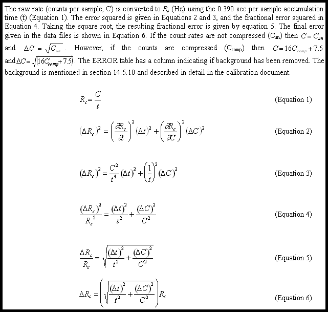 Equations 14-1 to 14-6
14.5.5 Quality Flags Flags assessing the quality of the data are based on operational housekeeping alarms, but in the future additional ones may need to be added which are based on on orbit and attitude, and additional calculations. All current flags are stored in a table extension. 14.5.6 Thruster Firings As mentioned earlier the calibrated (level 3) code reorganizes the thruster data into a table where each column refers to a given thruster name and each row is the start time of the thruster firing. The numbers under each thruster column indicate the duration of the thruster firings. Each thruster column has a title that looks like GC1_A2_FIRING where GC1 indicates it originated in a G&C packet, and FIRE indicates thruster firing. The thruster names are A1, A2, B1, B2, B3, C1, C2, C3, C4, D1, D2, D3, D4, F1, and F2. The value for each thruster firing corresponds to the duration of the thruster firing (0=0msec,1=5msec,2=20msec,3=40msec). In the raw data each row is a major frame, and the columns are minor frames where each minor frame is 40msecs. Thus, there are 25 columns with numbers between 0 and 24. In the level 3 (calibrated) data we calculate the start time of the firings for a given minor frame which means we have already taken the major frame start time and added in the time to the start of the minor frame where the firing occurred ( Start_time = major_frame_start_time + 0.040 * [minor_frame_number +1] ). The implication of this is that one row in the raw file may result in several rows in the calibrated file if there are multiple thruster firings. 14.5.7 SPICE Orbit and Attitude Calculations Our orbit and attitude calculations are contained in the SPICE_ORBIT_ATTITUDE_CALC extension. We calculate times for each SWAP measurement in the REAL_TIME extension. The MET for the packet is listed along with the UTC, and ET for the start and stop time of each measurement. There are two start times and two stop times one since each packet stores two measurements one in the first half second (labeled with a 0) and one in the second half second (labeled with a 1). In the tail the spacecraft is spinning so we have included the angle in the Xsc-Zsc plane between the Zsc axis and Jupiter's spin axis (north). This angle is 0 deg (90 deg) when Zsc (Xsc) is aligned with the North end of Jupiter's spin axis. These angles are named ANGLE_JSP_XZ in the files and calculations were done for the start, middle, and stop for each observation, since the spacecraft rotates quickly (5RPM). All other parameters are calculated at the middle of each observation. We also calculated the angle between the Ysc and the Sun, Jupiter, and Earth. The label for the angle between Ysc and the Sun for the 1st measurement is called Y_SUN_ANG0_MIDDLE. The distances from the spacecraft to Earth, Jupiter and the Sun are calculated (i.e., SUN_SC_0_MIDDLE). We calculate the angle to the Sun is in the X-Y plane (phi), and the latitude angle from the X-Y plane (theta). Positive phi values are toward the +Xsc axis and negative phi angles are towards the -Xsc axis. Negative theta values are towards the top of the instrument since the -Zsc axis is at the top of the instrument. Note this is the opposite convention used in the calibration chamber. However, the phi angle is analogous to the roll angle in calibration (see calibration Document). We also calculate the position and velocity of the spacecraft in IAU Jupiter Cartesian coordinates. The naming convention is such that the X component of position in IAU Jupiter for the 1st half second measurement is labeled as SC_IAU_JUP_X_0. Likewise the X component of the velocity is SC_IAU_JUP_VX_0. In addition to IAU Jupiter coordinates we calculate the spacecraft position in J2000 Jupiter coordinates the X component for the 1st measurement is labeled as SC_J2000_JUP_X_0. Column name descriptions are given in the header for the SPICE extension as well as the names of the SPICE kernel files used to perform the calculations.
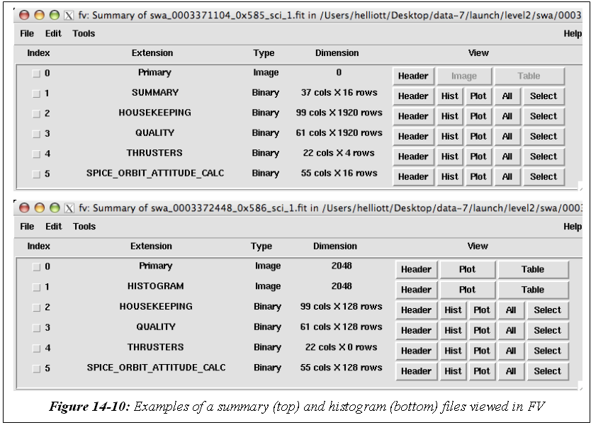 Figure 14-10: Examples of a summary (top) and histogram (bottom) files
viewed in FV
14.5.8 Summary and Histogram Files
Both the summary (Figure 14-10 top) and histogram (Figure 14-10 bottom)
files also have the primary header, and housekeeping, quality, thruster and
spice orbit attitude extensions the same as in the real-time files. In
extension 1 are is the summary data table converted to engineering units.
The histogram data are stored as images in the 0th and 1st extensions. The
0th extension contains the number of times data was added to each bin, and
the 1st extension contains the histogram count rates.
14.5.9 Calibration
Analysis of ground calibration data provides critical information used to
process the SWAP data, and is consequently a crucial input to our software;
therefore, details describing the use of calibration information in the
pipeline is described in section the calibration Document. The SWAP lab
calibration consists of an effective area; an angular response function for
the ESA (function of alpha and phi); an energy response curve for the RPA
that depends on the RPA and deflector voltages; a function representing how
the RPA changes the energy of ions prior to enter the ESA; an energy
response function for the ESA; the functions for how the width and center of
the ESA passband varies with alpha; and a function for how the conversion
factor for converting ESA voltage to energy depends on phi. Our pipeline
incorporates ESA and RPA response curves by precalculating the energy
passband for each RPA and ESA voltage pair stored in the onboard tables.
This information is used as a lookup table in the pipeline code so that each
RPA and ESA voltage step can be assigned a energy per charge value. The code
determines which set of tables to use by examining the time range since we
have had different sets of RPA and ESA tables loaded at different times in
the mission. To determine which of the 4 RPA tables to use the code compares
the sweep and plan number in the data to the sweep and plan number in the
precalculated tables. The results of the pipeline energy determination are
stored in the energy axis label extension and can be used directly to label
the y-axis of the spectrogram.
Figure 14-10: Examples of a summary (top) and histogram (bottom) files
viewed in FV
14.5.8 Summary and Histogram Files
Both the summary (Figure 14-10 top) and histogram (Figure 14-10 bottom)
files also have the primary header, and housekeeping, quality, thruster and
spice orbit attitude extensions the same as in the real-time files. In
extension 1 are is the summary data table converted to engineering units.
The histogram data are stored as images in the 0th and 1st extensions. The
0th extension contains the number of times data was added to each bin, and
the 1st extension contains the histogram count rates.
14.5.9 Calibration
Analysis of ground calibration data provides critical information used to
process the SWAP data, and is consequently a crucial input to our software;
therefore, details describing the use of calibration information in the
pipeline is described in section the calibration Document. The SWAP lab
calibration consists of an effective area; an angular response function for
the ESA (function of alpha and phi); an energy response curve for the RPA
that depends on the RPA and deflector voltages; a function representing how
the RPA changes the energy of ions prior to enter the ESA; an energy
response function for the ESA; the functions for how the width and center of
the ESA passband varies with alpha; and a function for how the conversion
factor for converting ESA voltage to energy depends on phi. Our pipeline
incorporates ESA and RPA response curves by precalculating the energy
passband for each RPA and ESA voltage pair stored in the onboard tables.
This information is used as a lookup table in the pipeline code so that each
RPA and ESA voltage step can be assigned a energy per charge value. The code
determines which set of tables to use by examining the time range since we
have had different sets of RPA and ESA tables loaded at different times in
the mission. To determine which of the 4 RPA tables to use the code compares
the sweep and plan number in the data to the sweep and plan number in the
precalculated tables. The results of the pipeline energy determination are
stored in the energy axis label extension and can be used directly to label
the y-axis of the spectrogram.
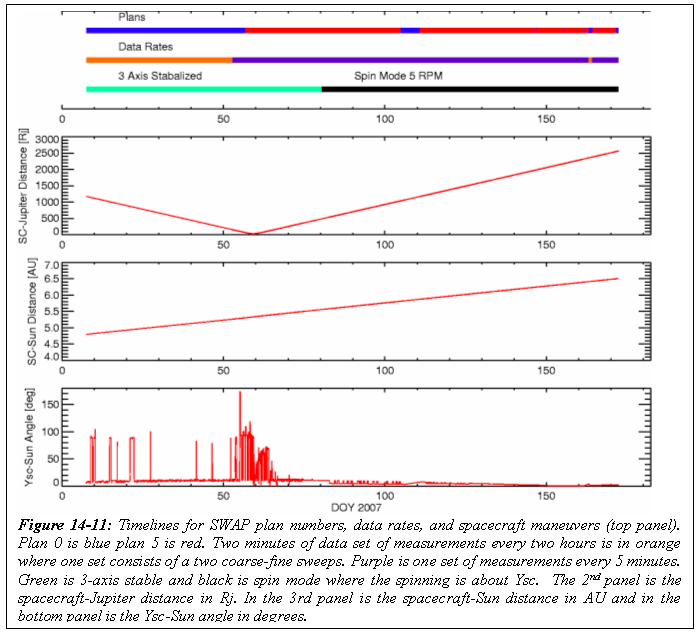 Figure 14-11: Timelines for SWAP plan numbers, data rates, and spacecraft
maneuvers (top panel). Plan 0 is blue plan 5 is red. Two minutes of data set
of measurements every two hours is in orange where one set consists of a two
coarse-fine sweeps. Purple is one set of measurements every 5 minutes. Green
is 3-axis stable and black is spin mode where the spinning is about Ysc.
The 2nd panel is the spacecraft-Jupiter distance in Rj. In the 3rd panel is
the spacecraft-Sun distance in AU, and in the bottom panel is the Ysc-Sun
angle in degrees.
14.5.10 Background Subtraction
There is a background in our data when the RPA is on. The background
reduces as the distance from the Sun increases and will most likely not be a
problem for the Pluto encounter. We can operate using only the ESA and have
done so for the Jupiter encounter (plan 5). For the solar wind measurements
inbound we needed to use the RPA (plan 0) to shield the instrument from high
solar wind fluxes. Background subtraction information is processed in
similar way as to the energy bin information. A given background is
subtraction is only valid for a given time range; therefore, a list of
background files and validity times are read in and then the background is
subtracted. The background files are stored in the calibration directory and
the names of the files used are stored in the list file. The instrument
detector gain will evolve with time and this information will be
incorporated in fashion similar to the background subtraction. Gain
calibrations occur during annual checkouts. The background subtraction is
described in more detail in the calibration Document
14.6 Operations
Plan 3 was used to take the first complete sweeps of the solar wind during
SWAP-009-6 in commissioning. The voltage tables were updated before the
beginning of the Jupiter phase to improve the voltage sweeps for the Jupiter
phase. There are only two plans used in the Jupiter phase plan 0 and plan 5.
Plan 0 is designed for the solar wind and plan 5 is designed for the
magnetosphere. The voltage settings in plan 0 protect the instrument from
high solar wind proton fluxes. Early on the data rate was such that two
coarse-fine scans were taken approximately every two hours. The spacing was
only approximately every two hours the operations were commanded and the
commands were adjusted by so as not to interfere with other instruments. At
2/21/2007 17:27:31 we kept the plan number set at 0 and then changed the
data rate such that we took 1 coarse and 1 fine scan every 5 minutes. Then
at 02/25/2007 19:22:43 we switched to plan 5, which consists two coarse
scans in 64 seconds every 5 minutes. In plan 5 the RPA is off and only the
ESA voltage is swept. With the RPA off, the instrument is so sensitive that
the high proton fluxes in the solar wind near Jupiter would cause the
instrument to automatically shut down. Since the instrument is more
sensitive in plan 5, we took some measurements in plan 0 in the
magnetosphere to insure that some measurements would be obtained even if the
spacecraft entered the solar wind. We show timelines for operations
in Figure 14-11 along with the distance to Jupiter and the Sun. And in the
bottom panel we show the angle between Ysc and the Sun. In spin mode the
spacecraft spins about Ysc. The spacecraft entered the magnetosphere on day
056(02/25) in 2007 and the first time it exited in the tail was
approximately on day 132(05/12) of 2007. There were many tail crossing and
there appears to be a boundary layer inside the sheath; therefore,
definitive boundary crossing times are difficult to determine. When SWAP
turned off on day168 (06/17) of 2007 for hibernation, New Horizons was once
again in the magnetosphere
14.7 Observation Examples
In this section we show two examples of SWAP data taken during the Jupiter
encounter. Figure 14-12 shows most of the solar wind measurements on
approach to Jupiter. The format is that of a color-coded spectrogram of the
background-subtracted coincidence count rates in Hz of solar wind ions as a
function energy per charge (E/q) as measured by the Solar Wind Around Pluto
(SWAP) instrument on New Horizons at ~4.9 AU from the Sun (~0.4 AU upstream
from Jupiter). We used plan 0 for these measurements since this plan helps
protect the instrument from high fluxes. In plan 0 the RPA is on at energies
below 2000 eV/q. The RPA creates a background and this background has been
removed (see calibration document). The lower trace shows the solar wind
protons, while the upper trace shows the alpha particles (He++), with
enhanced sensitivity (~100x larger) above 2 keV/q. Solar wind speed is a
function E/q, with 1 keV protons corresponding to typical, ~440 km/s solar
wind and larger (smaller) E/q representing faster (slower) wind speeds.
Interplanetary shocks passed over the New Horizons spacecraft at ~1800 on
Day-of-Year (DOY) 11 and at ~1300 on DOY 14 causing the abrupt jumps in
solar wind speed; the speed immediately following the latter shock was in
excess of 600 km/s. The slowly decreasing speed after the second shock
(falling E/q of the proton and alpha beams) is a rarefaction region, which
forms as faster solar wind outruns the slower solar wind behind it. In all,
these SWAP observations show a clear solar wind stream structure.
Below we show magnetospheric observations taken using plan 5 since plan 5 is
more sensitive and the flux rates are lower in the magnetosphere than in the
solar wind (Figure 14-13). The only time the plan 5 data has any background
is when there is penetrating radiation, and we do not remove any background
due to penetrating radiation. The penetrating radiation occurs close to
Jupiter and usually is greatest in the secondary and primary signals. When
it occurs, the count rates are usually elevated at all energy steps;
therefore, in spectrograms the penetrating radiation usually shows up as
vertical stripes. The penetrating radiation is significantly reduced in the
coincidence signal. The plan 5 data consists of one measurement set every
5th SWAP minute, and one set consists of 2 coarse scans performed in 64
seconds.
Figure 14-11: Timelines for SWAP plan numbers, data rates, and spacecraft
maneuvers (top panel). Plan 0 is blue plan 5 is red. Two minutes of data set
of measurements every two hours is in orange where one set consists of a two
coarse-fine sweeps. Purple is one set of measurements every 5 minutes. Green
is 3-axis stable and black is spin mode where the spinning is about Ysc.
The 2nd panel is the spacecraft-Jupiter distance in Rj. In the 3rd panel is
the spacecraft-Sun distance in AU, and in the bottom panel is the Ysc-Sun
angle in degrees.
14.5.10 Background Subtraction
There is a background in our data when the RPA is on. The background
reduces as the distance from the Sun increases and will most likely not be a
problem for the Pluto encounter. We can operate using only the ESA and have
done so for the Jupiter encounter (plan 5). For the solar wind measurements
inbound we needed to use the RPA (plan 0) to shield the instrument from high
solar wind fluxes. Background subtraction information is processed in
similar way as to the energy bin information. A given background is
subtraction is only valid for a given time range; therefore, a list of
background files and validity times are read in and then the background is
subtracted. The background files are stored in the calibration directory and
the names of the files used are stored in the list file. The instrument
detector gain will evolve with time and this information will be
incorporated in fashion similar to the background subtraction. Gain
calibrations occur during annual checkouts. The background subtraction is
described in more detail in the calibration Document
14.6 Operations
Plan 3 was used to take the first complete sweeps of the solar wind during
SWAP-009-6 in commissioning. The voltage tables were updated before the
beginning of the Jupiter phase to improve the voltage sweeps for the Jupiter
phase. There are only two plans used in the Jupiter phase plan 0 and plan 5.
Plan 0 is designed for the solar wind and plan 5 is designed for the
magnetosphere. The voltage settings in plan 0 protect the instrument from
high solar wind proton fluxes. Early on the data rate was such that two
coarse-fine scans were taken approximately every two hours. The spacing was
only approximately every two hours the operations were commanded and the
commands were adjusted by so as not to interfere with other instruments. At
2/21/2007 17:27:31 we kept the plan number set at 0 and then changed the
data rate such that we took 1 coarse and 1 fine scan every 5 minutes. Then
at 02/25/2007 19:22:43 we switched to plan 5, which consists two coarse
scans in 64 seconds every 5 minutes. In plan 5 the RPA is off and only the
ESA voltage is swept. With the RPA off, the instrument is so sensitive that
the high proton fluxes in the solar wind near Jupiter would cause the
instrument to automatically shut down. Since the instrument is more
sensitive in plan 5, we took some measurements in plan 0 in the
magnetosphere to insure that some measurements would be obtained even if the
spacecraft entered the solar wind. We show timelines for operations
in Figure 14-11 along with the distance to Jupiter and the Sun. And in the
bottom panel we show the angle between Ysc and the Sun. In spin mode the
spacecraft spins about Ysc. The spacecraft entered the magnetosphere on day
056(02/25) in 2007 and the first time it exited in the tail was
approximately on day 132(05/12) of 2007. There were many tail crossing and
there appears to be a boundary layer inside the sheath; therefore,
definitive boundary crossing times are difficult to determine. When SWAP
turned off on day168 (06/17) of 2007 for hibernation, New Horizons was once
again in the magnetosphere
14.7 Observation Examples
In this section we show two examples of SWAP data taken during the Jupiter
encounter. Figure 14-12 shows most of the solar wind measurements on
approach to Jupiter. The format is that of a color-coded spectrogram of the
background-subtracted coincidence count rates in Hz of solar wind ions as a
function energy per charge (E/q) as measured by the Solar Wind Around Pluto
(SWAP) instrument on New Horizons at ~4.9 AU from the Sun (~0.4 AU upstream
from Jupiter). We used plan 0 for these measurements since this plan helps
protect the instrument from high fluxes. In plan 0 the RPA is on at energies
below 2000 eV/q. The RPA creates a background and this background has been
removed (see calibration document). The lower trace shows the solar wind
protons, while the upper trace shows the alpha particles (He++), with
enhanced sensitivity (~100x larger) above 2 keV/q. Solar wind speed is a
function E/q, with 1 keV protons corresponding to typical, ~440 km/s solar
wind and larger (smaller) E/q representing faster (slower) wind speeds.
Interplanetary shocks passed over the New Horizons spacecraft at ~1800 on
Day-of-Year (DOY) 11 and at ~1300 on DOY 14 causing the abrupt jumps in
solar wind speed; the speed immediately following the latter shock was in
excess of 600 km/s. The slowly decreasing speed after the second shock
(falling E/q of the proton and alpha beams) is a rarefaction region, which
forms as faster solar wind outruns the slower solar wind behind it. In all,
these SWAP observations show a clear solar wind stream structure.
Below we show magnetospheric observations taken using plan 5 since plan 5 is
more sensitive and the flux rates are lower in the magnetosphere than in the
solar wind (Figure 14-13). The only time the plan 5 data has any background
is when there is penetrating radiation, and we do not remove any background
due to penetrating radiation. The penetrating radiation occurs close to
Jupiter and usually is greatest in the secondary and primary signals. When
it occurs, the count rates are usually elevated at all energy steps;
therefore, in spectrograms the penetrating radiation usually shows up as
vertical stripes. The penetrating radiation is significantly reduced in the
coincidence signal. The plan 5 data consists of one measurement set every
5th SWAP minute, and one set consists of 2 coarse scans performed in 64
seconds.
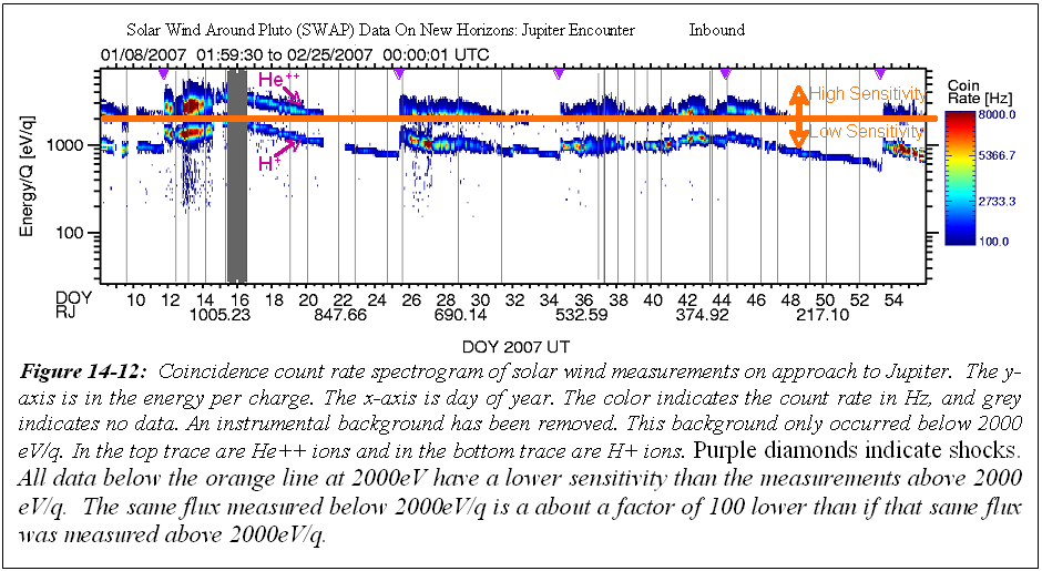 Figure 14-12: Coincidence count rate spectrogram of solar wind measurements
on approach to Jupiter. The y-axis is in the energy per charge. The x-axis
is day of year. The color indicates the count rate in Hz, and grey indicates
no data. An instrumental background has been removed. This background only
occurred below 2000 eV/q. In the top trace are He++ ions and in the bottom
trace are H+ ions. Purple diamonds indicate shocks. All data below the
orange line at 2000eV have a lower sensitivity than the measurements above
2000 eV/q. The same flux measured below 2000eV/q is a about a factor of 100
lower than if that same flux was measured above 2000eV/q.
14.8 Updates to Level 3 (calibrated data)
We added the center energy for given RPA and ESA voltages to the REAL_TIME
data extension. The column names are ENERGY_0 and ENERGY_1 in eV and
correspond to the 1st and 2nd measurement in a given packet (row). We
corrected the background subtraction. We corrected a rounding error in the
time used to calculate the spin angles in the SPICE extension and fixed a
small offset in the times for the spectrogram in the TIME_LABEL_SPECT
extension. We include directories of 1 day and 10 day coincidence
spectrograms plots for the entire Jupiter phase.
Figure 14-12: Coincidence count rate spectrogram of solar wind measurements
on approach to Jupiter. The y-axis is in the energy per charge. The x-axis
is day of year. The color indicates the count rate in Hz, and grey indicates
no data. An instrumental background has been removed. This background only
occurred below 2000 eV/q. In the top trace are He++ ions and in the bottom
trace are H+ ions. Purple diamonds indicate shocks. All data below the
orange line at 2000eV have a lower sensitivity than the measurements above
2000 eV/q. The same flux measured below 2000eV/q is a about a factor of 100
lower than if that same flux was measured above 2000eV/q.
14.8 Updates to Level 3 (calibrated data)
We added the center energy for given RPA and ESA voltages to the REAL_TIME
data extension. The column names are ENERGY_0 and ENERGY_1 in eV and
correspond to the 1st and 2nd measurement in a given packet (row). We
corrected the background subtraction. We corrected a rounding error in the
time used to calculate the spin angles in the SPICE extension and fixed a
small offset in the times for the spectrogram in the TIME_LABEL_SPECT
extension. We include directories of 1 day and 10 day coincidence
spectrograms plots for the entire Jupiter phase.
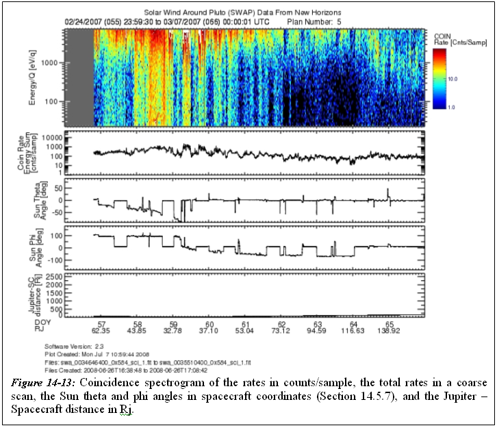 Figure 14-13: Coincidence spectrogram of the rates in counts/sample, the
total rates in a coarse scan, the Sun theta and phi angles in spacecraft
coordinates (Section 14.5.7), and the Jupiter to Spacecraft distance in Rj.
SWAP Science Goals
==================
These level 3 (calibrated) data products described above will allow us to
meet two key science goals as outlined in section 6.3.1.1 of the SWAP
Specification document (Document No. 05310-03-SWAPSPEC-01). Below we quote
this section.
The Mission Science Requirements document specifies that SWAP should make
the following measurements.
- Measure solar wind standoff to ~ 3000 km.
- Determine nature of solar wind interaction at Pluto. Distinguish
between magnetic, cometary, & ionospheric interactions.
14.8.1 Dataflow Block Diagram
Figure 14-13: Coincidence spectrogram of the rates in counts/sample, the
total rates in a coarse scan, the Sun theta and phi angles in spacecraft
coordinates (Section 14.5.7), and the Jupiter to Spacecraft distance in Rj.
SWAP Science Goals
==================
These level 3 (calibrated) data products described above will allow us to
meet two key science goals as outlined in section 6.3.1.1 of the SWAP
Specification document (Document No. 05310-03-SWAPSPEC-01). Below we quote
this section.
The Mission Science Requirements document specifies that SWAP should make
the following measurements.
- Measure solar wind standoff to ~ 3000 km.
- Determine nature of solar wind interaction at Pluto. Distinguish
between magnetic, cometary, & ionospheric interactions.
14.8.1 Dataflow Block Diagram
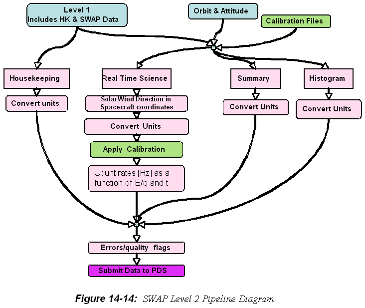 Figure 14-14 SWAP Level 2 Pipeline Diagram
14.8.2 Extra FITS Extensions and Their Definitions
We have binary tables for both real-time, and summary data. Likewise, we
have binary table extensions for housekeeping data, flags, errors, and
thruster packet spacecraft data. We have image extensions for both count
rate spectrograms and error spectrograms image. For histogram data we have
two image extensions: one for counts and one for accumulations (number of
samples).
14.8.3 Scientific Units
The level 3 calibrated code will have rate spectrogram in Hz, and all the
engineering data converted to engineering units.
14.8.4 Additional FITS and PDS Keywords Added
TBA
14.8.5 Hardware/OS Development Platform
Intel, Linux
14.8.6 Language(s) Used
C/C++
14.8.7 Third Party Libraries Required
Cfitsio and CSPICE.
14.8.8 Memory Required
TBA
14.8.9 Temporary File System Space Needed
None
14.8.10 Predicted Size of Output File(s)
TBA
14.8.11 Predicted Execution time
On the order of seconds
14.8.12 Contact/Support Person(s)
PI: Dave McComas
Lead Engineer and Project Manager: Scott Weidner
Onboard Software and Commanding: John Hanley
Pipeline and Science Operations: Heather Elliott
Sequencing: Helen Hart
14.8.13 Maintenance Schedule (Code/Data Updates, Documentation)
TBD
14.9 Packet Description
This section gives the parameters found in SWAP science packets. The names
are as given in the APL spreadsheets used to view the data in real-time and
playback modes. The level 1 names are shortened versions of these names.
REAL_TIME
=========
SWAP_RT.CC_PID_VER Primary Header - Version Number
SWAP_RT.CC_PID_TYPE Primary Header - Packet Type
SWAP_RT.CC_PID_SEC_FLAG Primary Header - Secondary Header Flag
SWAP_RT.CC_PID_APID Primary Header - Application ID; type of data ie
real-time, housekeeping, etc
SWAP_RT.CC_PSC_GRP_FLAG Primary Header - Grouping Flag; set to a
constant value, not used
SWAP_RT.CC_PSC_SSC Primary Header - Sequence Count
SWAP_RT.CC_PKT_DATA_LN Primary Header - Packet Length; this is used to
SWAP_RT.CC_MET_TIME Secondary Header - Time
SWAP_RT.SEC64_ST A bit indicating the beginning
of a 64-second cycle
SWAP_RT.PLAN_ID Plan ID
SWAP_RT.SWEEP_ID Sweep ID
SWAP_RT.ANGLE Commanded angle for deflection compensation
SWAP_RT.RPA_LVL0 RPA level during first half-second
SWAP_RT.DFL_LVL0 DFL level during first half-second
SWAP_RT.ESA_LVL0 ESA level during first half-second
SWAP_RT.RPA_LVL1 RPA level during first half-second
SWAP_RT.DFL_LVL1 DFL level during first half-second
SWAP_RT.ESA_LVL1 ESA level during first half-second
SWAP_RT.MODE Enumerated type representing each of the modes
SWAP_RT.PCEM_RNG_ST0 PCEM counts are compressed or raw during first
half-second; this is a flag that determines
if the data in SWAP_RT.PCEM_CNT0 is compressed
or not. If this flag is set to zero the data
are not compressed. If the flag is set to 1
then the data in SWAP_RT.PCEM_CNT0 is 1/16 of
the actual count rate.
SWAP_RT.SCEM_RNG_ST0 SCEM counts are compressed or raw
during first half-second
SWAP_RT.COIN_RNG_ST0 Coincidence counts are compressed or raw
during first half-second
SWAP_RT.PCEM_RNG_ST1 PCEM counts are compressed or
raw during second half-second
SWAP_RT.SCEM_RNG_ST1 SCEM counts are compressed or
raw during second half-second
SWAP_RT.COIN_RNG_ST1 Coincidence counts are compressed or
raw during second half-second
SWAP_RT.PCEM_CNT0 PCEM count value during first half-second
SWAP_RT.SCEM_CNT0 SCEM count value during first half-second
SWAP_RT.COIN_CNT0 Coincidence count value during first half-second
SWAP_RT.PCEM_CNT1 PCEM count value during second half-second
SWAP_RT.SCEM_CNT1 SCEM count value during second half-second
SWAP_RT.COIN_CNT1 Coincidence count value during second half-second
SWAP_RT.CHKSUM XOR checksum; this value is based on all the
other real-time quantities listed above.
It is used to determine if a bit was flipped
in one of the real-time quantities. If check
sum is not what is predicted based on the other
real-time quantities then the data need to be
thrown away.
SUMMARY
=======
SWAP_SM.CC_PID_VER Primary Header - Version Number
SWAP_SM.CC_PID_TYPE Primary Header - Packet Type
SWAP_SM.CC_PID_SEC_FLAG Primary Header - Secondary Header Flag
SWAP_SM.CC_PID_APID Primary Header - Application ID
SWAP_SM.CC_PSC_GRP_FLAG Primary Header - Grouping Flag
SWAP_SM.CC_PSC_SSC Primary Header - Sequence Count
SWAP_SM.CC_PKT_DATA_LN Primary Header - Packet Length
SWAP_SM.CC_MET_TIME Secondary Header - Time
SWAP_SM.BEG_TIME Time stamp at the beginning of this summary period
SWAP_SM.END_TIME The time stamp at the end of this summary period
SWAP_SM.N64_CNT Number of 64-second sample sets used
SWAP_SM.NDFL DFL
SWAP_SM.ANGLE_SUM Angle
SWAP_SM.DENSITY_SUM An estimate of the pseudo density
SWAP_SM.VELOCITY_SUM An estimate of the pseudo speed using energy
SWAP_SM.TEMP_SUM Estimate of the pseudo temperature
SWAP_SM.ANGLE_SSQ_HI The variance of the angles
SWAP_SM.ANGLE_SSQ_LO The variance of the angles
SWAP_SM.DENSITY_SSQ_HI The variance of the pseudo n-values
SWAP_SM.DENSITY_SSQ_LO The variance of the pseudo n-values
SWAP_SM.VELOCITY_SSQ_HI The variance of the pseudo V-values
SWAP_SM.VELOCITY_SSQ_LO The variance of the pseudo V-values
SWAP_SM.TEMP_SSQ_HI The variance of the pseudo T-values
SWAP_SM.TEMP_SSQ_LO The variance of the pseudo T-values
SWAP_SM.ANGLE_MIN Minimum Angle
SWAP_SM.DENSITY_MIN Minimum pseudo density
SWAP_SM.VELOCITY_MIN Minimum pseudo speed
SWAP_SM.TEMP_MIN Minimum pseudo Temperature
SWAP_SM.ANGLE_MAX Maximum Angle
SWAP_SM.DENSITY_MAX Maximum pseudo density
SWAP_SM.VELOCITY_MAX Maximum pseudo speed
SWAP_SM.TEMP_MAX Maximum pseudo temperature
SWAP_SM.CHKSUM XOR checksum
HISTOGRAM Type 1
================
SWAP_H0.CC_PKT_DATA_LN Primary Header - Packet Length
SWAP_H0.CC_MET_TIME Secondary Header - Time
SWAP_H0.BEG_TIME Time stamp at the beginning of
this histogram period
SWAP_H0.END_TIME The time stamp at the end of this histogram period
SWAP_H0.SMPLS_CNT Number of 64-second samples used
SWAP_H0.PLAN_ID The Plan ID used for the
current science sweeping mode
SWAP_H0.TABLE_ID Table ID within the Plan ID that is being used
SWAP_H0.SEQNUM_CNT Sequence number starting at 0 for header
SWAP_H0.DATA Histogram data
SWAP_H0.CHKSUM XOR checksum
HISTOGRAM Type 2
================
SWAP_H1.CC_PID_VER Primary Header - Version Number
SWAP_H1.CC_PID_TYPE Primary Header - Packet Type
SWAP_H1.CC_PID_SEC_FLAG Primary Header - Secondary Header Flag
SWAP_H1.CC_PID_APID Primary Header - Application ID
SWAP_H1.CC_PSC_GRP_FLAG Primary Header - Grouping Flag
SWAP_H1.CC_PSC_SSC Primary Header - Sequence Count
SWAP_H1.CC_PKT_DATA_LN Primary Header - Packet Length
SWAP_H1.CC_MET_TIME Secondary Header - Time
SWAP_H1.SEQNUM_CNT Sequence number
SWAP_H1.DATA Histogram data
SWAP_H1.CHKSUM XOR checksum starting with
beginning of CCSDS header
HOUSEKEEPING
============
SWAP_HK.CC_PID_VER Primary Header - Version Number
SWAP_HK.CC_PID_TYPE Primary Header - Packet Type
SWAP_HK.CC_PID_SEC_FLAG Primary Header - Secondary Header Flag
SWAP_HK.CC_PID_APID Primary Header - Application ID
SWAP_HK.CC_PSC_GRP_FLAG Primary Header - Grouping Flag
SWAP_HK.CC_PSC_SSC Primary Header - Sequence Count
SWAP_HK.CC_PKT_DATA_LN Primary Header - Packet Length
SWAP_HK.CC_MET_TIME Secondary Header - Time
SWAP_HK.CMD_EXE_CNT Cumulative mod-256 count of
successfully executed commands
SWAP_HK.CMD_REJ_CNT Cumulative mod-256 count of rejected commands
SWAP_HK.LUT_CHOICE Which LUT is in use
SWAP_HK.PCEM_SAFE PCEM was safed due to CEM interrupts
SWAP_HK.SCEM_SAFE SCEM was safed due to CEM interrupts
SWAP_HK.WDT_ST SWAP has rebooted due to a watchdog expiration.
SWAP_HK.RCV_SAFE_ST SWAP has received safe command from S/C
SWAP_HK.SAFE_ST SWAP has safed itself.
SWAP_HK.PCEM_RATE_ST Count rate threshold for PCEM
counter has been exceeded
SWAP_HK.SCEM_RATE_ST Count rate threshold for the SCEM
counter has been exceeded
SWAP_HK.PCEM_CURR_ST Current threshold for the PCEM has been exceeded
SWAP_HK.SCEM_CURR_ST Current threshold for the SCEM has been exceeded
SWAP_HK.PCEM_VOLT_ST Voltage tolerance for the PCEM has been exceeded.
SWAP_HK.SCEM_VOLT_ST Voltage tolerance for the SCEM has been exceeded.
SWAP_HK.LVPS_VOLT_ST Voltage tolerance for +5 V or -5V supply
has been exceeded.
SWAP_HK.LVPS_CURR_ST Current tolerance for +5 V or -5V supply
has been exceeded.
SWAP_HK.OVR_TEMP_ST Upper temperature limit exceeded.
SWAP_HK.UND_TEMP_ST Lower temperature limit exceeded.
SWAP_HK.MODE Enumerated type representing each of the modes
SWAP_HK.MEMDP_ST MEMDUMP State
SWAP_HK.SENSOR_TEMP Temperature of sensor detector. AD mux = 0x10
SWAP_HK.HVSUPP_TEMP Temperature of HVPS. AD mux = 0x11
SWAP_HK.CNTRLR_TEMP Temperature of controller. AD mux = 0x12
SWAP_HK.PCEM_VOLT Voltage monitor of PCEM high-voltage
power supply. AD mux = 0x02
SWAP_HK.SCEM_VOLT Voltage monitor of SCEM high-voltage
power supply. AD mux = 0x03
SWAP_HK.PCEM_CURR Strip current monitor of PCEM high-voltage
power supply. AD mux = 0x04
SWAP_HK.SCEM_CURR Strip current monitor of SCEM high-voltage
power supply. AD mux = 0x05
SWAP_HK.P5_VOLT Voltage monitor of +5V power supply.
AD mux = 0x0c
SWAP_HK.N5_VOLT Voltage monitor of -5V power supply.
AD mux = 0x0d
SWAP_HK.P5_CURR Current monitor of +5V power supply.
AD mux = 0x0e
SWAP_HK.N5_CURR Current monitor of -5V power supply.
AD mux = 0x0f
SWAP_HK.SWAP_REV Revision number for the SWAP software
SWAP_HK.LAST_OPCODE Opcode of last executed command
SWAP_HK.PHD_LLD_LVL DAC Level of PHD LLD
SWAP_HK.MEMLD_ST MEMLOAD state
SWAP_HK.OPT1_ST State of primary optics
SWAP_HK.OPT2_ST State of backup optics
SWAP_HK.PCEM_ST State of Primary Channel Electron
Multiplier disable/enable
SWAP_HK.SCEM_ST State of Secondary Channel Electron disable/enable
SWAP_HK.SPARE1 SPARE
SWAP_HK.PCEM_CNT_ST The PCEM count rate was tripped
but handled by SWAPFW
SWAP_HK.SCEM_CNT_ST The SCEM count rate was tripped
but handled by SWAPFW
SWAP_HK.PCEM_CURRTHR Current level when PCEM safety algos are tripped
SWAP_HK.SCEM_CURRTHR Current level when SCEM safety algos are tripped
SWAP_HK.PCEM_LVL PCEM DAC level
SWAP_HK.SCEM_LVL SCEM DAC level
SWAP_HK.AGND_VOLT Voltage monitor of Analog ground. A/D mux = 0x00
SWAP_HK.CEM_CURR Current level when SCEM safety
interrupt is tripped
SWAP_HK.ESA1_VOLT Voltage monitor of ESA high-voltage
power supply. AD mux = 0x06
SWAP_HK.ESA2_VOLT Voltage monitor of ESA high-voltage
power supply. AD mux = 0x07
SWAP_HK.DFL1_VOLT Voltage monitor of DFL high-voltage
power supply. AD mux = 0x08
SWAP_HK.DFL2_VOLT Voltage monitor of DFL high-voltage
power supply. AD mux = 0x09
SWAP_HK.RPA1_VOLT Voltage monitor of RPA high-voltage
power supply. AD mux = 0x0a
SWAP_HK.RPA2_VOLT Voltage monitor of RPA high-voltage
power supply. AD mux = 0x0b
SWAP_HK.P2_5_VOLT Voltage monitor of +2.5V reference. AD mux = 0x13
SWAP_HK.PHD_LLD_VOLT Voltage monitor of PHD_LLD. Ad mux = 0x14
SWAP_HK.PCEM_RATELIM The count value at which the
primary CEM safety limit is set.
SWAP_HK.SCEM_RATELIM The count value at which the
secondary CEM safety limit is set.
SWAP_HK.STIM_ENA State of whether the stimultor
pulsers are enabled or disabled.
SWAP_HK.PPS_SEL_ST State of which side of the IEM
interface is being used.
SWAP_HK.PPS_DET_ST 1 PPS detected state
SWAP_HK.CEM_INT_LIM Current limit at which the CEM
triggers an interrupt.
SWAP_HK.CMD_ECHO_ST Whether command echo is enabled or disabled
SWAP_HK.HV_PGSAFE_ST State of safe / arm plug
SWAP_HK.HV_PGENA_ST State of high-voltage disable/enable plug
SWAP_HK.HV_ARM_ST State of high-voltage software disable/enable
SWAP_HK.CEM_INT_DIP Counts to dip the CEM supplies
SWAP_HK.PLAN_ID The Plan ID used for the current
science sweeping mode if any.
SWAP_HK.SWEEP_ID Current Sweep table ID
SWAP_HK.ANGLE The commanded angle for deflection compensation
SWAP_HK.PCEM_VLT1_ST PCEM voltage is out of tolerance
for only one 0.5 second sample
SWAP_HK.PCEM_CUR1_ST PCEM current is out of tolerance
for only one 0.5 second sample
SWAP_HK.SCEM_VLT1_ST SCEM voltage is out of tolerance
for only one 0.5 second sample
SWAP_HK.SCEM_CUR1_ST SCEM current is out of tolerance
for only one 0.5 second sample
SWAP_HK.PCEM_INT_ST The CEM current interrupt was tripped,
but handled by SWAPFW
SWAP_HK.SCEM_INT_ST The CEM current interrupt was tripped,
but handled by SWAPFW
SWAP_HK.EEP2_RDY EEPROM 2 is ready to be written
SWAP_HK.EEP1_RDY EEPROM 1 is ready to be written
SWAP_HK.FPGA_TYPE Type number of the FPGA
SWAP_HK.FPGA_REV Revision number of the FPGA
SWAP_HK.SM_TLM How often the science summary packet is output.
SWAP_HK.HX_TLM How often the histogram
telemetry packet is output.
SWAP_HK.RT_TLM How often all of the 64-second
real-time packets are output
SWAP_HK.HK_TLM How often the housekeeping packet is output.
SWAP_HK.FPGA_PUP_ST A status of the power on check
of the FPGA initialization check
SWAP_HK.EEPL2_CKS_ST Status of the power on check
of the EEP_L2 checksum
SWAP_HK.EEPL1_CKS_ST Status of the power on check
of EEP_L1 checksum
SWAP_HK.RAM_D_ST Status of the power on check
of the RAM_D memory test
SWAP_HK.EEPC2_CKS_ST Status of the power on check
of the EEP_C2 checksum
SWAP_HK.EEPC1_CKS_ST Status of the power on check
of the EEP_C1 checksum
SWAP_HK.RAM_C_ST Status of the power on check
of the RAM_C memory test
SWAP_HK.PROM_CKS_ST Status of the power on check
of the PROM checksum
SWAP_HK.CHKSUM XOR checksum
Figure 14-14 SWAP Level 2 Pipeline Diagram
14.8.2 Extra FITS Extensions and Their Definitions
We have binary tables for both real-time, and summary data. Likewise, we
have binary table extensions for housekeeping data, flags, errors, and
thruster packet spacecraft data. We have image extensions for both count
rate spectrograms and error spectrograms image. For histogram data we have
two image extensions: one for counts and one for accumulations (number of
samples).
14.8.3 Scientific Units
The level 3 calibrated code will have rate spectrogram in Hz, and all the
engineering data converted to engineering units.
14.8.4 Additional FITS and PDS Keywords Added
TBA
14.8.5 Hardware/OS Development Platform
Intel, Linux
14.8.6 Language(s) Used
C/C++
14.8.7 Third Party Libraries Required
Cfitsio and CSPICE.
14.8.8 Memory Required
TBA
14.8.9 Temporary File System Space Needed
None
14.8.10 Predicted Size of Output File(s)
TBA
14.8.11 Predicted Execution time
On the order of seconds
14.8.12 Contact/Support Person(s)
PI: Dave McComas
Lead Engineer and Project Manager: Scott Weidner
Onboard Software and Commanding: John Hanley
Pipeline and Science Operations: Heather Elliott
Sequencing: Helen Hart
14.8.13 Maintenance Schedule (Code/Data Updates, Documentation)
TBD
14.9 Packet Description
This section gives the parameters found in SWAP science packets. The names
are as given in the APL spreadsheets used to view the data in real-time and
playback modes. The level 1 names are shortened versions of these names.
REAL_TIME
=========
SWAP_RT.CC_PID_VER Primary Header - Version Number
SWAP_RT.CC_PID_TYPE Primary Header - Packet Type
SWAP_RT.CC_PID_SEC_FLAG Primary Header - Secondary Header Flag
SWAP_RT.CC_PID_APID Primary Header - Application ID; type of data ie
real-time, housekeeping, etc
SWAP_RT.CC_PSC_GRP_FLAG Primary Header - Grouping Flag; set to a
constant value, not used
SWAP_RT.CC_PSC_SSC Primary Header - Sequence Count
SWAP_RT.CC_PKT_DATA_LN Primary Header - Packet Length; this is used to
SWAP_RT.CC_MET_TIME Secondary Header - Time
SWAP_RT.SEC64_ST A bit indicating the beginning
of a 64-second cycle
SWAP_RT.PLAN_ID Plan ID
SWAP_RT.SWEEP_ID Sweep ID
SWAP_RT.ANGLE Commanded angle for deflection compensation
SWAP_RT.RPA_LVL0 RPA level during first half-second
SWAP_RT.DFL_LVL0 DFL level during first half-second
SWAP_RT.ESA_LVL0 ESA level during first half-second
SWAP_RT.RPA_LVL1 RPA level during first half-second
SWAP_RT.DFL_LVL1 DFL level during first half-second
SWAP_RT.ESA_LVL1 ESA level during first half-second
SWAP_RT.MODE Enumerated type representing each of the modes
SWAP_RT.PCEM_RNG_ST0 PCEM counts are compressed or raw during first
half-second; this is a flag that determines
if the data in SWAP_RT.PCEM_CNT0 is compressed
or not. If this flag is set to zero the data
are not compressed. If the flag is set to 1
then the data in SWAP_RT.PCEM_CNT0 is 1/16 of
the actual count rate.
SWAP_RT.SCEM_RNG_ST0 SCEM counts are compressed or raw
during first half-second
SWAP_RT.COIN_RNG_ST0 Coincidence counts are compressed or raw
during first half-second
SWAP_RT.PCEM_RNG_ST1 PCEM counts are compressed or
raw during second half-second
SWAP_RT.SCEM_RNG_ST1 SCEM counts are compressed or
raw during second half-second
SWAP_RT.COIN_RNG_ST1 Coincidence counts are compressed or
raw during second half-second
SWAP_RT.PCEM_CNT0 PCEM count value during first half-second
SWAP_RT.SCEM_CNT0 SCEM count value during first half-second
SWAP_RT.COIN_CNT0 Coincidence count value during first half-second
SWAP_RT.PCEM_CNT1 PCEM count value during second half-second
SWAP_RT.SCEM_CNT1 SCEM count value during second half-second
SWAP_RT.COIN_CNT1 Coincidence count value during second half-second
SWAP_RT.CHKSUM XOR checksum; this value is based on all the
other real-time quantities listed above.
It is used to determine if a bit was flipped
in one of the real-time quantities. If check
sum is not what is predicted based on the other
real-time quantities then the data need to be
thrown away.
SUMMARY
=======
SWAP_SM.CC_PID_VER Primary Header - Version Number
SWAP_SM.CC_PID_TYPE Primary Header - Packet Type
SWAP_SM.CC_PID_SEC_FLAG Primary Header - Secondary Header Flag
SWAP_SM.CC_PID_APID Primary Header - Application ID
SWAP_SM.CC_PSC_GRP_FLAG Primary Header - Grouping Flag
SWAP_SM.CC_PSC_SSC Primary Header - Sequence Count
SWAP_SM.CC_PKT_DATA_LN Primary Header - Packet Length
SWAP_SM.CC_MET_TIME Secondary Header - Time
SWAP_SM.BEG_TIME Time stamp at the beginning of this summary period
SWAP_SM.END_TIME The time stamp at the end of this summary period
SWAP_SM.N64_CNT Number of 64-second sample sets used
SWAP_SM.NDFL DFL
SWAP_SM.ANGLE_SUM Angle
SWAP_SM.DENSITY_SUM An estimate of the pseudo density
SWAP_SM.VELOCITY_SUM An estimate of the pseudo speed using energy
SWAP_SM.TEMP_SUM Estimate of the pseudo temperature
SWAP_SM.ANGLE_SSQ_HI The variance of the angles
SWAP_SM.ANGLE_SSQ_LO The variance of the angles
SWAP_SM.DENSITY_SSQ_HI The variance of the pseudo n-values
SWAP_SM.DENSITY_SSQ_LO The variance of the pseudo n-values
SWAP_SM.VELOCITY_SSQ_HI The variance of the pseudo V-values
SWAP_SM.VELOCITY_SSQ_LO The variance of the pseudo V-values
SWAP_SM.TEMP_SSQ_HI The variance of the pseudo T-values
SWAP_SM.TEMP_SSQ_LO The variance of the pseudo T-values
SWAP_SM.ANGLE_MIN Minimum Angle
SWAP_SM.DENSITY_MIN Minimum pseudo density
SWAP_SM.VELOCITY_MIN Minimum pseudo speed
SWAP_SM.TEMP_MIN Minimum pseudo Temperature
SWAP_SM.ANGLE_MAX Maximum Angle
SWAP_SM.DENSITY_MAX Maximum pseudo density
SWAP_SM.VELOCITY_MAX Maximum pseudo speed
SWAP_SM.TEMP_MAX Maximum pseudo temperature
SWAP_SM.CHKSUM XOR checksum
HISTOGRAM Type 1
================
SWAP_H0.CC_PKT_DATA_LN Primary Header - Packet Length
SWAP_H0.CC_MET_TIME Secondary Header - Time
SWAP_H0.BEG_TIME Time stamp at the beginning of
this histogram period
SWAP_H0.END_TIME The time stamp at the end of this histogram period
SWAP_H0.SMPLS_CNT Number of 64-second samples used
SWAP_H0.PLAN_ID The Plan ID used for the
current science sweeping mode
SWAP_H0.TABLE_ID Table ID within the Plan ID that is being used
SWAP_H0.SEQNUM_CNT Sequence number starting at 0 for header
SWAP_H0.DATA Histogram data
SWAP_H0.CHKSUM XOR checksum
HISTOGRAM Type 2
================
SWAP_H1.CC_PID_VER Primary Header - Version Number
SWAP_H1.CC_PID_TYPE Primary Header - Packet Type
SWAP_H1.CC_PID_SEC_FLAG Primary Header - Secondary Header Flag
SWAP_H1.CC_PID_APID Primary Header - Application ID
SWAP_H1.CC_PSC_GRP_FLAG Primary Header - Grouping Flag
SWAP_H1.CC_PSC_SSC Primary Header - Sequence Count
SWAP_H1.CC_PKT_DATA_LN Primary Header - Packet Length
SWAP_H1.CC_MET_TIME Secondary Header - Time
SWAP_H1.SEQNUM_CNT Sequence number
SWAP_H1.DATA Histogram data
SWAP_H1.CHKSUM XOR checksum starting with
beginning of CCSDS header
HOUSEKEEPING
============
SWAP_HK.CC_PID_VER Primary Header - Version Number
SWAP_HK.CC_PID_TYPE Primary Header - Packet Type
SWAP_HK.CC_PID_SEC_FLAG Primary Header - Secondary Header Flag
SWAP_HK.CC_PID_APID Primary Header - Application ID
SWAP_HK.CC_PSC_GRP_FLAG Primary Header - Grouping Flag
SWAP_HK.CC_PSC_SSC Primary Header - Sequence Count
SWAP_HK.CC_PKT_DATA_LN Primary Header - Packet Length
SWAP_HK.CC_MET_TIME Secondary Header - Time
SWAP_HK.CMD_EXE_CNT Cumulative mod-256 count of
successfully executed commands
SWAP_HK.CMD_REJ_CNT Cumulative mod-256 count of rejected commands
SWAP_HK.LUT_CHOICE Which LUT is in use
SWAP_HK.PCEM_SAFE PCEM was safed due to CEM interrupts
SWAP_HK.SCEM_SAFE SCEM was safed due to CEM interrupts
SWAP_HK.WDT_ST SWAP has rebooted due to a watchdog expiration.
SWAP_HK.RCV_SAFE_ST SWAP has received safe command from S/C
SWAP_HK.SAFE_ST SWAP has safed itself.
SWAP_HK.PCEM_RATE_ST Count rate threshold for PCEM
counter has been exceeded
SWAP_HK.SCEM_RATE_ST Count rate threshold for the SCEM
counter has been exceeded
SWAP_HK.PCEM_CURR_ST Current threshold for the PCEM has been exceeded
SWAP_HK.SCEM_CURR_ST Current threshold for the SCEM has been exceeded
SWAP_HK.PCEM_VOLT_ST Voltage tolerance for the PCEM has been exceeded.
SWAP_HK.SCEM_VOLT_ST Voltage tolerance for the SCEM has been exceeded.
SWAP_HK.LVPS_VOLT_ST Voltage tolerance for +5 V or -5V supply
has been exceeded.
SWAP_HK.LVPS_CURR_ST Current tolerance for +5 V or -5V supply
has been exceeded.
SWAP_HK.OVR_TEMP_ST Upper temperature limit exceeded.
SWAP_HK.UND_TEMP_ST Lower temperature limit exceeded.
SWAP_HK.MODE Enumerated type representing each of the modes
SWAP_HK.MEMDP_ST MEMDUMP State
SWAP_HK.SENSOR_TEMP Temperature of sensor detector. AD mux = 0x10
SWAP_HK.HVSUPP_TEMP Temperature of HVPS. AD mux = 0x11
SWAP_HK.CNTRLR_TEMP Temperature of controller. AD mux = 0x12
SWAP_HK.PCEM_VOLT Voltage monitor of PCEM high-voltage
power supply. AD mux = 0x02
SWAP_HK.SCEM_VOLT Voltage monitor of SCEM high-voltage
power supply. AD mux = 0x03
SWAP_HK.PCEM_CURR Strip current monitor of PCEM high-voltage
power supply. AD mux = 0x04
SWAP_HK.SCEM_CURR Strip current monitor of SCEM high-voltage
power supply. AD mux = 0x05
SWAP_HK.P5_VOLT Voltage monitor of +5V power supply.
AD mux = 0x0c
SWAP_HK.N5_VOLT Voltage monitor of -5V power supply.
AD mux = 0x0d
SWAP_HK.P5_CURR Current monitor of +5V power supply.
AD mux = 0x0e
SWAP_HK.N5_CURR Current monitor of -5V power supply.
AD mux = 0x0f
SWAP_HK.SWAP_REV Revision number for the SWAP software
SWAP_HK.LAST_OPCODE Opcode of last executed command
SWAP_HK.PHD_LLD_LVL DAC Level of PHD LLD
SWAP_HK.MEMLD_ST MEMLOAD state
SWAP_HK.OPT1_ST State of primary optics
SWAP_HK.OPT2_ST State of backup optics
SWAP_HK.PCEM_ST State of Primary Channel Electron
Multiplier disable/enable
SWAP_HK.SCEM_ST State of Secondary Channel Electron disable/enable
SWAP_HK.SPARE1 SPARE
SWAP_HK.PCEM_CNT_ST The PCEM count rate was tripped
but handled by SWAPFW
SWAP_HK.SCEM_CNT_ST The SCEM count rate was tripped
but handled by SWAPFW
SWAP_HK.PCEM_CURRTHR Current level when PCEM safety algos are tripped
SWAP_HK.SCEM_CURRTHR Current level when SCEM safety algos are tripped
SWAP_HK.PCEM_LVL PCEM DAC level
SWAP_HK.SCEM_LVL SCEM DAC level
SWAP_HK.AGND_VOLT Voltage monitor of Analog ground. A/D mux = 0x00
SWAP_HK.CEM_CURR Current level when SCEM safety
interrupt is tripped
SWAP_HK.ESA1_VOLT Voltage monitor of ESA high-voltage
power supply. AD mux = 0x06
SWAP_HK.ESA2_VOLT Voltage monitor of ESA high-voltage
power supply. AD mux = 0x07
SWAP_HK.DFL1_VOLT Voltage monitor of DFL high-voltage
power supply. AD mux = 0x08
SWAP_HK.DFL2_VOLT Voltage monitor of DFL high-voltage
power supply. AD mux = 0x09
SWAP_HK.RPA1_VOLT Voltage monitor of RPA high-voltage
power supply. AD mux = 0x0a
SWAP_HK.RPA2_VOLT Voltage monitor of RPA high-voltage
power supply. AD mux = 0x0b
SWAP_HK.P2_5_VOLT Voltage monitor of +2.5V reference. AD mux = 0x13
SWAP_HK.PHD_LLD_VOLT Voltage monitor of PHD_LLD. Ad mux = 0x14
SWAP_HK.PCEM_RATELIM The count value at which the
primary CEM safety limit is set.
SWAP_HK.SCEM_RATELIM The count value at which the
secondary CEM safety limit is set.
SWAP_HK.STIM_ENA State of whether the stimultor
pulsers are enabled or disabled.
SWAP_HK.PPS_SEL_ST State of which side of the IEM
interface is being used.
SWAP_HK.PPS_DET_ST 1 PPS detected state
SWAP_HK.CEM_INT_LIM Current limit at which the CEM
triggers an interrupt.
SWAP_HK.CMD_ECHO_ST Whether command echo is enabled or disabled
SWAP_HK.HV_PGSAFE_ST State of safe / arm plug
SWAP_HK.HV_PGENA_ST State of high-voltage disable/enable plug
SWAP_HK.HV_ARM_ST State of high-voltage software disable/enable
SWAP_HK.CEM_INT_DIP Counts to dip the CEM supplies
SWAP_HK.PLAN_ID The Plan ID used for the current
science sweeping mode if any.
SWAP_HK.SWEEP_ID Current Sweep table ID
SWAP_HK.ANGLE The commanded angle for deflection compensation
SWAP_HK.PCEM_VLT1_ST PCEM voltage is out of tolerance
for only one 0.5 second sample
SWAP_HK.PCEM_CUR1_ST PCEM current is out of tolerance
for only one 0.5 second sample
SWAP_HK.SCEM_VLT1_ST SCEM voltage is out of tolerance
for only one 0.5 second sample
SWAP_HK.SCEM_CUR1_ST SCEM current is out of tolerance
for only one 0.5 second sample
SWAP_HK.PCEM_INT_ST The CEM current interrupt was tripped,
but handled by SWAPFW
SWAP_HK.SCEM_INT_ST The CEM current interrupt was tripped,
but handled by SWAPFW
SWAP_HK.EEP2_RDY EEPROM 2 is ready to be written
SWAP_HK.EEP1_RDY EEPROM 1 is ready to be written
SWAP_HK.FPGA_TYPE Type number of the FPGA
SWAP_HK.FPGA_REV Revision number of the FPGA
SWAP_HK.SM_TLM How often the science summary packet is output.
SWAP_HK.HX_TLM How often the histogram
telemetry packet is output.
SWAP_HK.RT_TLM How often all of the 64-second
real-time packets are output
SWAP_HK.HK_TLM How often the housekeeping packet is output.
SWAP_HK.FPGA_PUP_ST A status of the power on check
of the FPGA initialization check
SWAP_HK.EEPL2_CKS_ST Status of the power on check
of the EEP_L2 checksum
SWAP_HK.EEPL1_CKS_ST Status of the power on check
of EEP_L1 checksum
SWAP_HK.RAM_D_ST Status of the power on check
of the RAM_D memory test
SWAP_HK.EEPC2_CKS_ST Status of the power on check
of the EEP_C2 checksum
SWAP_HK.EEPC1_CKS_ST Status of the power on check
of the EEP_C1 checksum
SWAP_HK.RAM_C_ST Status of the power on check
of the RAM_C memory test
SWAP_HK.PROM_CKS_ST Status of the power on check
of the PROM checksum
SWAP_HK.CHKSUM XOR checksum